Avicenna J Environ Health Eng. 10(2):85-97.
doi: 10.34172/ajehe.5283
Original Article
Performance of TANN, NARX, and GMDHT Models for Urban Water Demand Forecasting: A Case Study in a Residential Complex in Qom, Iran
Mostafa Rezaali 1  , Reza Fouladi-Fard 2, 3, * , Abdolreza Karimi 4
Author information:
1Department of Geography, University of Florida, Gainesville, Florida, United States
2Research Center for Environmental Pollutants, Department of Environmental Health Engineering, Qom University of Medical Sciences, Qom, Iran
3Environmental Health Research Center, School of Health and Nutrition, Lorestan University of Medical Sciences, Khorramabad, Iran
4Department of Civil Engineering, Qom University of Technology, Qom, Iran
Abstract
To keep the balance between demand and supply, methods based on the average per capita consumption were usually applied to predict water demand. More complicated models such as linear regression and time series models were developed for this purpose. However, after the introduction of artificial neural networks (ANNs), different applications of this method were used in the field of water supply management, especially for urban water demand prediction. In this study, multiple types of ANNs were studied to understand their suitability for a residential complex water demand prediction in the city of Qom, Iran. The results indicated that time series ANN (TANN), nonlinear autoregressive network with exogenous inputs (NARX), group method of data handling time series (GMDHT), and their wavelet counterparts (i.e., w-TANN and w-NARX) exhibited varying degrees of performance. Among the aforementioned models, w-NARX performed the best (based on the average overall error) with the test set root mean squared error (MSE) of 49.5 (m3/h) and R of 0.93, followed by the GMDHT model with the test set MSE of 104 (m3/h) and R of 0.97 and w-TANN with the test set MSE of 68.8 (m3/h) and R of 0.91. In addition, the feedback connection in NARX compared to TANN demonstrated overall performance improvement.
Keywords: Recurrent artificial neural networks, Group method of data handling, Time series modeling, Urban water demand forecasting, Qom,
Copyright and License Information
© 2023 The Author(s); Published by Hamadan University of Medical Sciences.
This is an open-access article distributed under the terms of the Creative Commons Attribution License (
https://creativecommons.org/licenses/by/4.0), which permits unrestricted use, distribution, and reproduction in any medium, provided the original work is properly cited.
Please cite this article as follows: Rezaali M, Fouladi-Fard R, Karimi A. Performance of TANN, NARX, and GMDHT models for urban water demand forecasting: a case study in a residential complex in Qom, Iran. Avicenna J Environ Health Eng. 2023; 10(2):85-97. doi: 10.34172/ ajehe.5283
1. Introduction
Many decades ago, satisfying consumer water demand with sufficient quality was one of the major concerns for water supply companies and utilities. According to the literature, predicting water demand can help to provide users with quality water in adequate volumes at reasonable pressure (1). The challenge of water demand prediction is of particular interest in arid/semi-arid cities, because of water shortages which usually occur in dry seasons (2). In the case of supervised learning, one of the most widely applied techniques used for training artificial neural network (ANN) is a back-propagation algorithm with feedforward networks. Maier and Dandy (3) argued that the geometry of ANNs is rarely addressed in the papers and network parameters like learning rate, transfer function, and error function were disregarded or rarely considered. It is also noteworthy to mention that the words “learning” and “training” in ANNs are equivalent to the parameter estimation phase in statistical models. Water demand prediction can have many benefits such as pressure management in the water distribution system and avoiding water leakages (1). Ghiassi et al(4) utilized the DAN2 model to predict short-term, medium-term, and long-term urban water demand and compared the performance of DAN2 with that of the ANN and autoregressive integrated moving average (ARIMA). The results indicated that the DAN2 model had better performance than ARIMA and ANN. Adamowski and Karapataki (5) compared multiple linear regression (MLR) and ANN for peak urban water demand forecasting in Nicosia. Different learning algorithms were evaluated for training the ANN model. The results suggested that the Levenberg–Marquardt algorithm provided a more accurate prediction than MLR and the other types of ANNs.
Over time, different architectures of ANN were developed. For example, feedforward networks have drawn lots of attention since the early stages of development. In this study, a nonlinear autoregressive network with exogenous inputs (NARX), NARX coupled with wavelet transform (w-NARX), time-delayed ANN (TANN) and its wavelet version (w-TANN), and group method of data handling time series (GMDHT) were trained to predict the daily water demand in Mahdie Residential Complex (MRC) in Qom, Iran.
2. Methods
2.1. Study Area
Qom (capital city of Qom province), one of the most populous cities in Iran, is located in the center of Iran with a semi-arid climate (6-9). Historically, the water supply of Qom has been of great importance due to the arid environment of this city and water scarcity. The first water distribution system of Qom was designed and constructed in 1964 by connecting four wells using 83 km cast iron pipes along the Qomrood River and pumping the water into the two elevated concrete tanks with a capacity of 2000 m3. After a while, with a growing population, the number of wells increased to 34. In 1994, 15 Khordad Dam was built to ensure the supply of standard drinkable water to the consumers. On average, in the summer season, the city’s water demand is estimated to be 4600 m3/s, but in the winter, this number decreases to 2900 m3/s (10). Therefore, the water demand for the whole city can potentially be a function of climatic parameters. Fig. 1 presents an aerial view of the study area.
The MRC is chosen as a case study due to its recent construction, low leakage rates, and its distinction as a separate pressure zone within the city. The water distribution network characteristics of the MRC in Iran are distinct due to the negligible impact of hydraulic difficulties on the urban water demand (UWD). Consequently, the flow rate data accurately represents the unadulterated UWD. According to the Ministry of Energy in Iran (2), the estimated daily per-capita water consumption of the MRC during the study period is around 288 L. This amount is approximately 68 L more than the national average and 12 L less than the water consumption in Tehran, the capital of Iran. The complex encompasses an expansive green space spanning over 2 km2 and accommodates over 3000 inhabitants, a significant portion of whom are those engaged in the profession of preaching Islam and cultural advocacy.
2.2. Technical Properties of the Distribution Network
The main water supply of the city is provided by Koucherey and 15 Khordad dams with a capacity of 207 and 165 MCM, respectively. Other water supply sources are groundwater, namely Aliabad wells and Qomrood wells. The water of MRC is supplied by a tank which is usually refilled every 24 hours.
2.3. Experimental Setup
The water flow data was received from the Water and Wastewater Company. The dataset is recorded every hour from May 13, 2016, to February 19, 2017, which is equal to a 6768-hour observation. Since there were only a few records of precipitation, rainfall occurrence, and amount were not used as explanatory inputs of the model.
The extraction of useful information from a large dataset has been thoroughly investigated in the literature (11). Input variable selection has been a significant challenge in any research related to the topic of prediction (12). To meet this challenge, the iterative input selection (IIS) algorithm was used to select the most relevant inputs describing the water demand dataset (13). This algorithm has proved to be capable of choosing the most appropriate and non-redundant input in several testing conditions (13).
2.4. Predictive Models
2.4.1. MLP Neural Network
One of the most widely applied architectures of ANNs is the multi-layer perceptron feedforward neural network (MFNN). This popularity may stem from the ability of MFNN to approximate any complex nonlinear system dynamics. This method is a supervised learning method that estimates and adjusts weights and biases to approximate the output from the given inputs. In each epoch, it reduces the error between the estimated and real output by minimizing the cost function. According to the literature, a three-layer MFNN (input layer, one hidden layer, and output layer) can approximate almost all types of system behavior (3,14).
Equation 1 and Equation 2 illustrate the mathematical basis of a three-layer MFNN (15).
Eq. (1)
Eq. (2)
where nH is hidden layer node, no is the output layer node, n1is the input layer node, xi(t) is the input to node i of the input layer, yi(t) is the quantity computed by node j of the hidden layer, and Zk(t) is the output computed by node k of the output layer. Wijh controls the strength of the connection between input node i and hidden node j controls the strength of the connection between hidden node j and output node k. Input and hidden layer bias are considered x0 = 1 and y0 = 1 to permit adjustment of the mean level at each stage.
24.1.1. TANN
The time series version of ANN (i.e., TANN) was used in this study. Hansen and Nelson (16) suggested that due to the ability of ANNs to deal with non-linear cyclic patterns, they are good alternatives to handle time-series variations (3). Considering a stationary neural network, a function to describe the relationship between inputs and outputs can be written as Equation 3:
Eq. (3)
where xn is an independent variable, and y is a dependent variable. It is considered that this type of ANN is functionally equivalent to non-linear regression models. However, to make an ANN extrapolate beyond the range of data, another function is needed to forecast future data based on past observation as an input. This is mathematically achieved by Equation 4:
Eq. (4)
where yt is the observation at time t. The t in the training process is called lag or tapped delays.
2.4.2. NARX
Historically, moving average (MA), autoregressive moving average (ARMA), and linear parametric autoregressive (AR) have been widely used among researchers and scientists. However, due to the linear nature of ARMA, it may not perfectly fit nonlinear time series systems (17,18). With the emergence of feedforward neural networks, it was found that by connecting each neuron to the next layer, the previous layer, the same layer, and even themselves (recurrent neural networks), they can implicitly model dynamical system properties (3). NARX neural networks are proven to learn the behavior of the system more efficiently. Compared to other network geometries, NARX neural networks generally converge faster and generalize better (19). It is a type of recurrent neural network that can capture both linear and nonlinear relationships between input and output data over time. NARX models are particularly useful when dealing with dynamic systems where the current output depends not only on past inputs and outputs but also on exogenous (external) inputs (20). The scheme of the NARX neural network with a feedback connection is shown in Fig. 2.
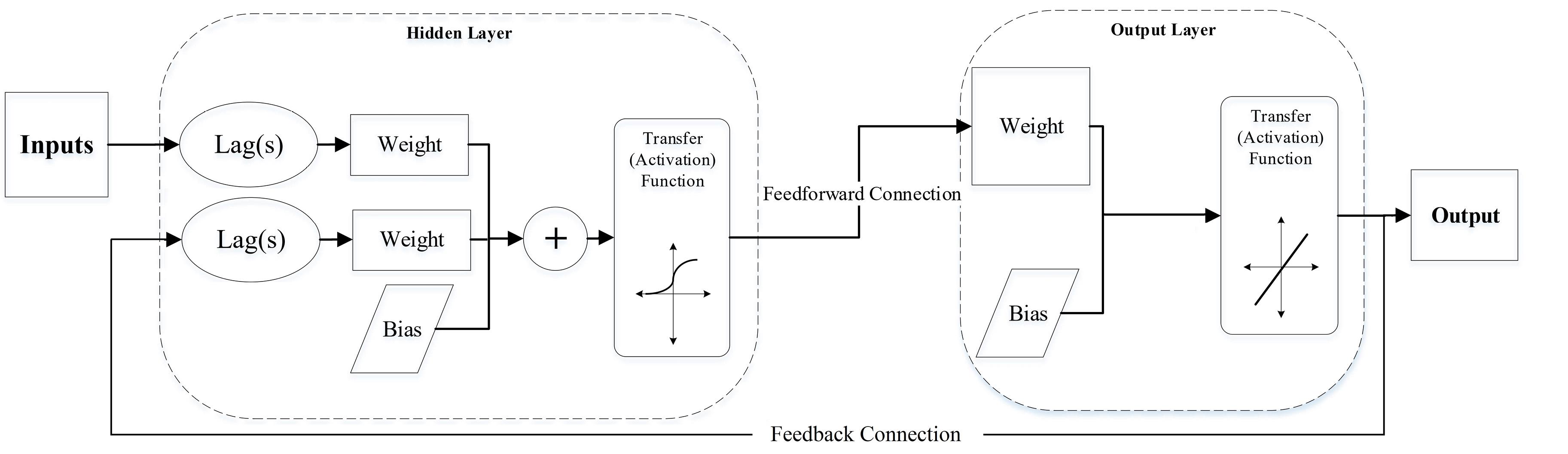
Fig. 2.
A NARX Network With a Feedback Connection
.
A NARX Network With a Feedback Connection
2.4.3. Wavelet Analysis
Wavelet analysis (WA) is a mathematical tool to extract specific information from data. These data are usually hard to interpret because of their chaotic structure. Examples of these data are noisy images, high-frequency signals, and perturbed time series data like Mackey-Glass chaotic time series, and so on.
WA has been applied to different types of applications, including but certainly not limited to signal de-noising, image processing, and time series decomposition with flying colors (21). The coupled form of wavelet analysis and neural networks has been widely used in different applications. However, many of these studies used wavelet transform (WT) functions incorrectly in terms of using future data when decomposing the time series data, selecting the level of decomposition and wavelet filters inappropriately, and data partitioning (22,23). To summarize, it is essential to carefully select the type of WT, wavelet filter and scaling, level of decomposition, and data partitioning.
2.4.4. GMDHT
GMDH algorithm is based on a category of the heuristic self-organizing method used in GMDH neural networks. Introduced by Ivakhnenko (24), GMDH is a technique for constructing an extremely high-order regression-type polynomial. This approach has the ability to establish a higher-level correlation for a user, based on the inputs and outputs of a system that is being analyzed by the user (25). In this study, the GMDH algorithm was used in MATLAB exactly based on the parameters which are defined by Ivakhnenko (26). Fig. 3 illustrates the general process of elimination of functions which describes the system dynamics less efficiently.
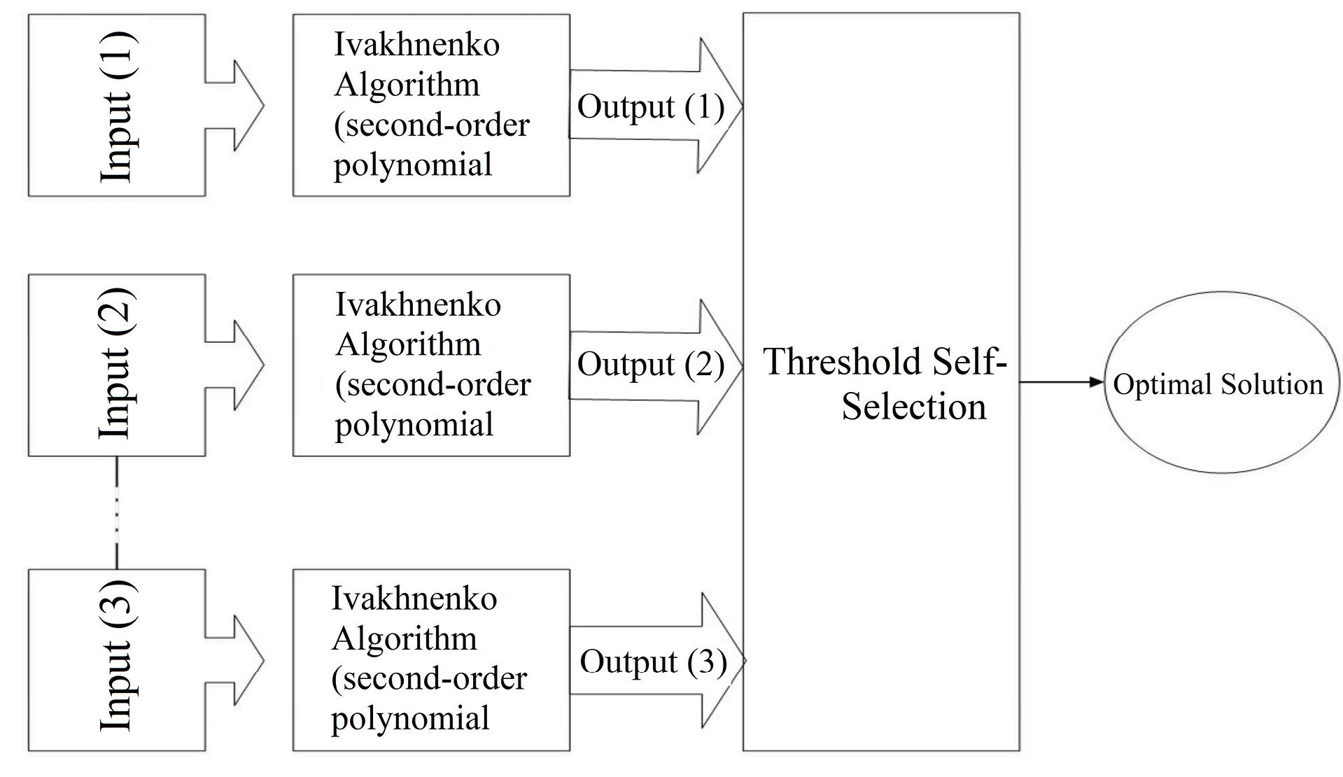
Fig. 3.
The General Process of the GMDH Neural Network
.
The General Process of the GMDH Neural Network
GMDH or multiple nonlinear regression can be used in different types of categories such as identification of physical laws, an approximation of multidimensional problems, pattern recognition, and so on (27).
GMDH neural network fits equation 5 (i.e., nonlinear polynomial regression of inputs as X and outputs as Y) where ɑ is the intercept, β is the coefficient, and k is the number of inputs or observations.
Eq. (5)
Although GMDH and multiple nonlinear regression are similar in terms of using nonlinear regression (MNLR), GMDH is different from MNLR. GMDH uses equation 5 to fit a regression to the target dataset. However, MNLR can use different types of nonlinear regressions. GMDH is a self-organizing method that applies the basic idea of a natural selection algorithm, while MNLR does not. It is also known as a polynomial neural network (28).
2.5. Model Development
Although there is no consensus about the optimal network architecture of ANNs, the importance of ANNs architecture in the performance of the model has never been questioned. Defining an optimal network architecture is one of the most challenging tasks in the modeling process. A reason for this might be that the performance of the neural networks is highly problem-dependent (3); therefore, it is hard to define architecture as a global solution. However, there are some general guidelines to achieve better performance using a specific ANN-based model. In the following subsections, the detailed description and structure of all applied models are discussed.
2.5.1. Model Geometry
2.5.1.1. Model Inputs, Data Division, and Choice of Lags
The input data, including maximum daily temperature, wind speed, and cloud cover were considered as the inputs of the ANN models. Having this in mind, before using these parameters as inputs, they all underwent one-sample Kolmogorov-Smirnov test to study the distribution of data. The test results for all of the parameters indicated that the test rejects the null hypothesis at the 5% significance level. This means the distribution of data does not follow the Gaussian distribution. Thus, the Spearman correlation analysis was performed to investigate the relationship of these parameters with water demand data.
Data division was performed by dividing data into three subsets: 70% for training, 15% for validation, and 15% for testing. Due to temporal dependencies of time series prediction, the data set was not shuffled before the training process (1,29); therefore, the sequence of data remained the same as the inputs.
Before the data was used as input for the training process, all data were normalized between specific ranges based on the domain of the transfer function used. It is noteworthy to mention that all the models used in this paper were scripted in MATLAB (version 2017a). Equation 6 provides mathematical formulae of the normalization used in this study:
Eq. (6)
where ymax is the maximum value for each row of y, ymin is the minimum value for each row of y, x is an N-by-Q matrix, xmin is the minimum value for each row of x, and xmax is the maximum value for each row of x.
2.5.1.2. Number of Hidden Layers and Nodes
Since the number of hidden layers and neurons is highly problem-dependent, there is no global number of layers of neurons to model the system dynamics. A high number of neurons can cause overtraining and produce unreliable performance results due to the inability of the model to generalize.
In this study, the number of layers and neurons was defined by a trial and error process. It was found that a network with one hidden layer and one neuron can approximate the input data efficiently.
2.5.1.3. Choice of Transfer (Activation) Function
Generally, the selection of transfer function is, to some extent, dependent on how much data are noisy and are highly non-linear (3). Since the weight initialization process in ANNs-based models is random, selecting the best model usually requires simulating the model multiple times and saving the model and its results for each simulation. To this end, the models were scripted in a way that in each simulation, the train, validation and test performance, outputs, and targets, and the NARX, wavelet-NARX (w-NARX), TANN, and wavelet-TANN (w-TANN) models are saved on the hard disk in a text file in space-delimited format. The number of the simulation was chosen by considering computational limitations. After 30 simulations, the best model was selected. This process was divided into four main combined network configurations with a hyperbolic tangent sigmoid and symmetric saturating linear transfer function, log-sigmoid and linear transfer function, hyperbolic tangent sigmoid and linear transfer function, and sigmoidal and symmetric saturating linear transfer function in the hidden layer and output layer, respectively.
In this study, to conform to the demand of the transfer function (30) and to avoid saturation of the transfer function (31), the model with tansig transfer function was evaluated by the scaled range of [-0.9 0.9], and the model with logsig transfer function was evaluated by the scaled range of [0.1 0.9]. Fig. 4 shows the transfer functions applied in this study to evaluate network performance.
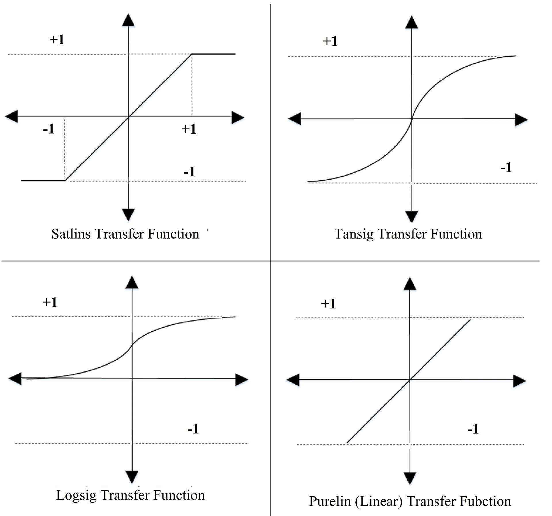
Fig. 4.
Transfer Functions Used to Evaluate Overall Network Performance
.
Transfer Functions Used to Evaluate Overall Network Performance
2.5.1.4. Choice of Optimization Method
In both of TANN and NARX models, the Levenberg–Marquardt algorithm (LMA) was selected to train the model. This algorithm is based on the classic Newton algorithm with some modifications. The changes in the behavior of this algorithm at a different distance of local minima error enable this algorithm to converge faster to global minima error and escape from local minima error. Using LMA has several advantages over other algorithms such as gradient descent with momentum (GD) and conjugate gradient (CG) (32-35).
2.5.2. Wavelet NARX and ANN
The framework used in this study is based on the wavelet data-driven forecasting framework (WDDFF) method introduced by Quilty and Adamowski (22). To this end, the following subsections define the procedure used to apply WDDFF.
2.5.2.1. Selection of WT
There are two types of widely used WT for hydrological prediction, which do not consider future data for decomposition, including maximal overlap discrete wavelet transform and à trous (AT). However, since AT can be used for preprocessing both target and input data, in this study the authors proposed this WT (22).
2.5.2.2. Selection of Decomposition Level and Wavelet Filters
Considering the number of data available, the maximum decomposition level was used based on boundary-affected coefficients (BAC) calculated by Equation 7:
where L is the maximum level of decomposition and S is the number of scaling coefficients. As the water demand data was available for 283 days, and BAC data were not to be used in the training process, selecting the correct number of L and S was very important. It was found that a Daubechies (db) filter of scale 3 and level 3 will provide sufficient data and efficiency (283–36 = 247) to train the network. The time series of the demanded data were decomposed by two filters: a low-pass filter to get approximation decomposition and a high-pass filter to get details of the signal decomposition. The data flow through the W-NARX and W-TANN is shown in Fig. 5.
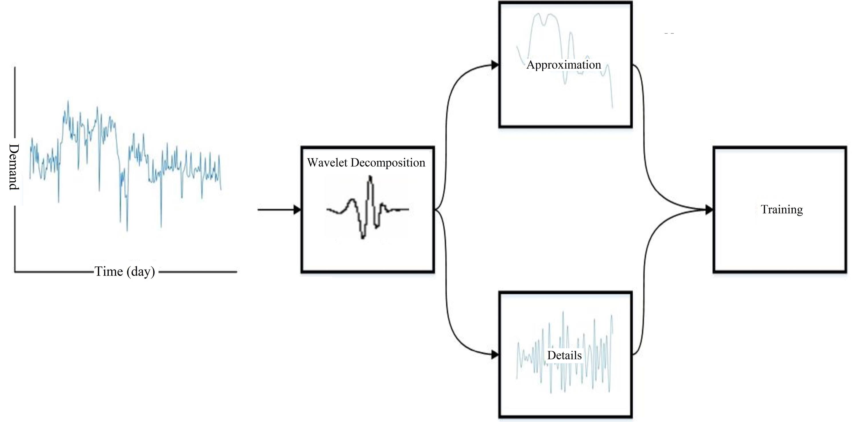
Fig. 5.
Data Flow in the W-NARX and W-TANN
.
Data Flow in the W-NARX and W-TANN
Before using the data, 36 records of each lagged dataset (1 to 14) were eliminated to remove BAC. After normalization between -1 to 1, data is fed into NARX as an input.
2.5.3. GMDH
The input parameters for training the model included demand data, temperature, cloud cover, and wind speed in the previous two weeks. To apply GMDH model regression to the data, the Time Series Prediction tool using GMDH in MATLAB was used (36). The number of neurons was optimized in an additive stepwise mode by adding a neuron to find which model could provide the best performance. Similarly, the method of choosing the best delay and threshold value was done by a trial and error process.
2.5.3.1. Data Division
The data were divided into two groups, including training and testing groups. The least-squares algorithm was used to train 70% of the input data, and the rest of the data set (30%) was used for testing.
2.5.4. Performance Evaluation Methods
All of the models underwent an identical performance evaluation process. Equations 8 and 9 were chosen to evaluate each model performance.
Eq. (8)
Eq. (9)
where, n is the number of test cases, Oi is the true value of the target variable for the case i, and Pi is the respective prediction of the model for the same case.
3. Results and Discussion
According to the IIS input selection, maximum daily temperature, wind speed, mean daily cloud cover, holidays, and rainfall amount were selected as input variables by IIS. Conversely, cloud cover was excluded as a potential input for the proposed models (Fig. 6)
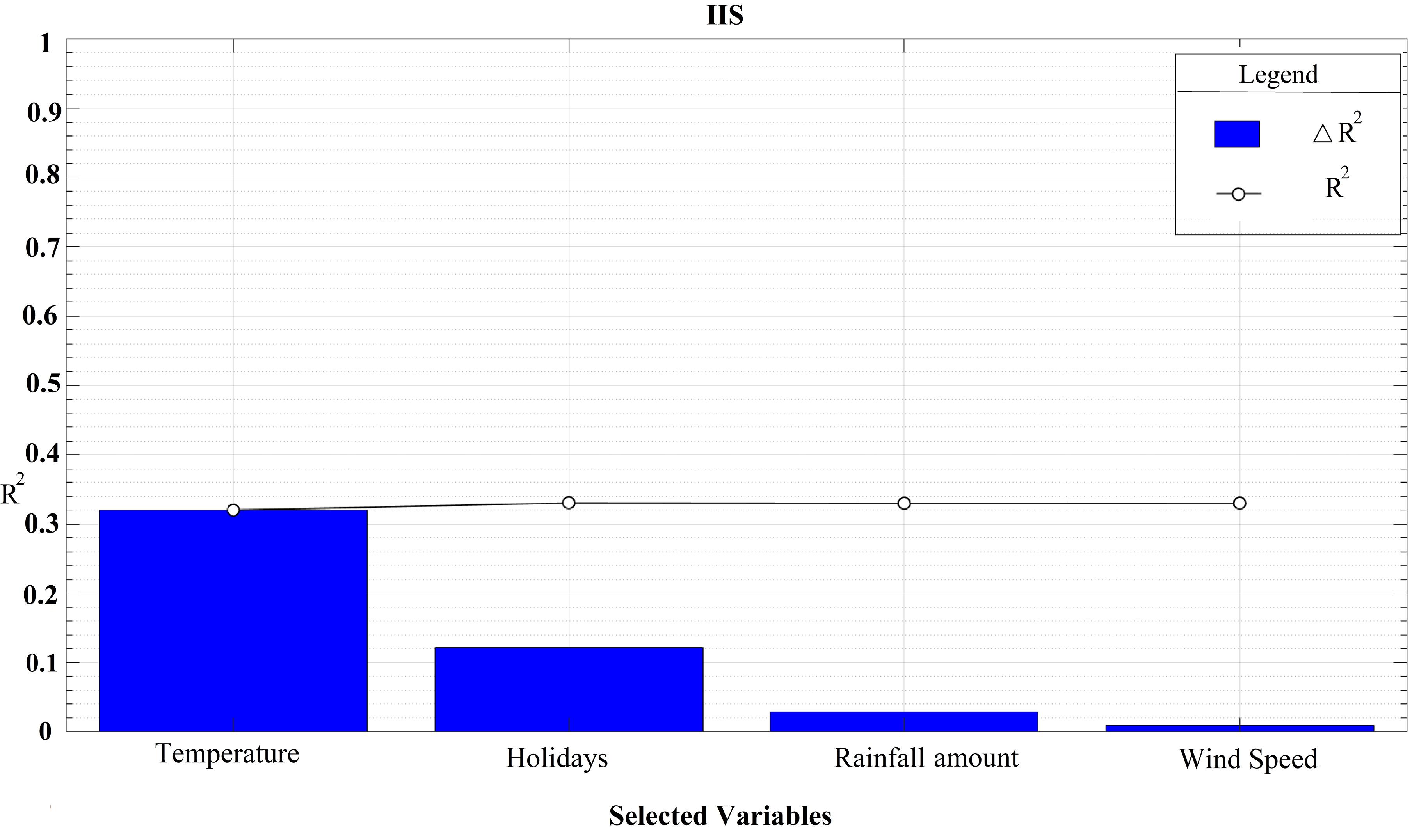
Fig. 6.
IIS Algorithm Output
.
IIS Algorithm Output
The technique of cross-correlation was employed to ascertain the temporal associations between the input variables and the data on water demand. This approach has been extensively employed in the determination of input delays (37-43). Fig. 7 shows the cross-correlation plot of the input variables and water demand data. Accordingly, rainfall amount at a time (t), wind speed at time (t), temperature at time (t-3), and holidays at time (t-14) had the highest correlation with the water demand observations. Similarly, Rezaali et al (2) found a significant correlation between temperature, holidays, and wind speed. Prasad et al (44) also implemented IIS for streamflow forecasting and found similar results. Both of these commonalities demonstrate the association between water flow rate and meteorological and calendar inputs.
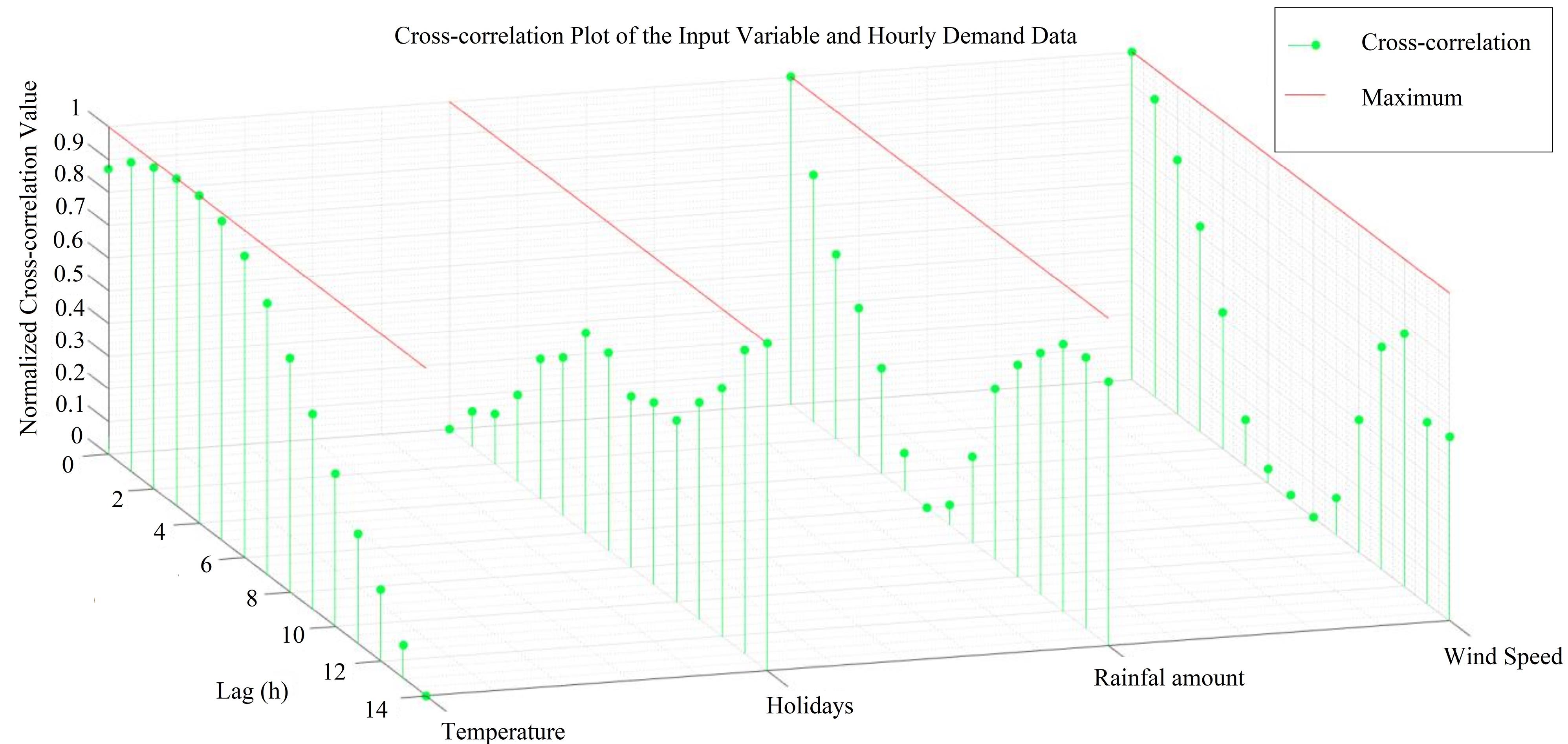
Fig. 7.
Cross-correlation Plot of the Input Variables
.
Cross-correlation Plot of the Input Variables
3.1. Model Performance
As Table 1 and Table 2 suggest, the performance of TANN models is better than NARX models in the training phase. However, in the validation and test phases, NARX performance, on average, was better than TANN.
Table 1.
Performance of the Best TANN Models with a Different Combination of the Transfer Function in the Hidden and Output Layers
|
Hidden Layer
|
Output Layer
|
Train (MSE)
|
Validation (MSE)
|
Test (MSE)
|
R2 Across All Data
|
| Logsig |
Purelin |
5.35E + 04 |
1.34E + 05 |
2.05E + 05 |
7.38E-01 |
| Tansig |
Satlins |
8.54E + 04 |
9.46E + 04 |
1.46E + 05 |
7.21E-01 |
| Logsig |
Satlins |
1.49E + 04a |
2.91E + 05 |
3.14E + 05 |
7.11E-01 |
| Tansig |
Purelin |
5.47E + 04 |
1.75E + 05 |
1.94E + 05 |
7.23E-01 |
a = indicates the lowest error in train, validation, and test, and the highest correlation coefficient.
Table 2.
Performance of the Best NARX Models with a Different Combination of the Transfer Function in the Hidden and Output Layers
|
Hidden Layer
|
Output Layer
|
Train (MSE)
|
Validation (MSE)
|
Test (MSE)
|
R2 Across All Data
|
| Logsig |
Purelin |
8.88E + 04 |
6.42E + 04 |
1.49E + 05 |
7.24E-01 |
| Tansig |
Satlins |
8.10E + 04a |
7.37E + 04 |
1.45E + 05 |
7.34E-01 |
| Logsig |
Satlins |
9.46E + 04 |
8.79E + 04 |
1.07E + 05 |
7.16E-01 |
| Tansig |
Purelin |
1.08E + 05 |
6.01E + 04 |
1.09E + 05 |
7.01E-01 |
a = indicates the lowest error in train, validation, and test, and the highest correlation coefficient.
The results of wavelet coupled networks in each combination after 30 runs are provided in Table 3.
Table 3.
Performance of the Best w-NARX Models with a Different Combination of the Transfer Function in the Hidden and Output Layers
|
Hidden Layer
|
Output Layer
|
Train (MSE)
|
Validation (MSE)
|
Test (MSE)
|
R2 Across All Data
|
MAPE
|
| Logsig |
Purelin |
2.66E + 03 |
2.50E + 03 |
2.83E + 03 |
8.72E-01 |
12.85% |
| Tansig |
Satlins |
2.76E + 03 |
2.39E + 03 |
2.82E + 03 |
8.70E-01 |
12.92% |
| Logsig |
Satlins |
2.57E + 03 |
2.28E + 03 |
2.45E + 03 |
8.80E-01 |
12.15% |
| Tansig |
Purelin |
2.81E + 03 |
2.16E + 03 |
2.65E + 03 |
8.70E-01 |
12.76% |
a = indicates the lowest error in train, validation, and test, and the highest correlation coefficient.
Although all of the w-NARX models performed similarly, the tansig-satlins model performed best. This network also had the best average train, validation, and test performance among other combinations of transfer functions.
To provide a measure to compare the results of this study with those of other studies, the w-TANN model was investigated with different combinations of transfer functions. Table 4 provides some information about the mentioned combinations. It is noteworthy to state that the best model was selected by 30 times of simulations for each transfer function combination.
Table 4.
Performance of Best w-TANN Models with a Different Combination of the Transfer Function in the Hidden and Output Layers
|
Hidden Layer
|
Output Layer
|
Train (MSE)
|
Validation (MSE)
|
Test (MSE)
|
R2 Across All Data
|
| Logsig |
Purelin |
3.14E + 03 |
5.55E + 03 |
6.32E + 03 |
8.10E-01 |
| Tansig |
Satlins |
3.38E + 03 |
4.20E + 03a |
4.41E + 03a |
8.24E-01 |
| Logsig |
Satlins |
3.04E + 03 |
4.74E + 03 |
5.29E + 03 |
8.26E-01 |
| Tansig |
Purelin |
2.86E + 03a |
4.85E + 03 |
4.74E + 03 |
8.35E-01 |
a = indicates the lowest error in train, validation, and test, and the highest correlation coefficient.
As Table 4 suggests, the models with tansig and purelin transfer functions in the hidden and output layers performed better than other combinations of transfer functions. Besides, by comparing these two tables, it will be evident that w-NARX models performed considerably better than w-TANN models. The reason for this could be the feedback connection in NARX models. The feedback connection may help the model to learn idiosyncrasies better than TANN does and therefore may help to learn the behavior of the consumers.
Heidari et al (45) found that NARX outperformed other models for the prediction of the spreading dynamics of different droplets on various substrates. In a similar case study of water demand prediction for 24 hours and 1 week, Bata et al (46) proposed that NARX model with correlated exogenous parameters dropped the error by 30% on average compared with a single-input model. It was also found that the length of the NARX training set had a negative correlation with the model performance for the above-mentioned lead time. This is in accordance with what was found in the current study, which is majorly due to the overfitting issue and the feedback connection in NARX models.
By trial and error, the configuration of the GMDHT was defined, that is: selection pressure lags, and train to test ratio. Compared to ANN-based time series models, GMDHT requires less time to fit nonlinear regression to the target data set. In this research, the GMDHT method was more consistent than the ANN model. This could be because of random weight initialization and other complexities related to ANN-based models. The results of the best GMDHT models with different configurations are provided in Table 5.
Table 5.
Best GMDHT Model Output Configuration Results
|
Model Num.
|
Selection Pressure
|
Max. Num. Layers
|
Number of Neurons
|
Train (MSE)
|
Test (MSE)
|
R2 Across All Data
|
| 1 |
0.6 |
3 |
5 |
3.19E + 04a |
1.09E + 04 |
9.33E-01 |
| 2 |
0.7 |
3 |
8 |
3.83E + 04 |
1.06E + 04 |
9.19E-01 |
| 3 |
0.8 |
4 |
12 |
4.19E + 04 |
1.47E + 04 |
9.03E-01 |
a = indicates the lowest error in train, validation, and test, and the highest correlation coefficient.
According to this table, the best GMDHT model was selected based on train, test, and R coefficient (i.e., model number 1). Compared to ANN-based models, w-NARX and some configurations of w-TANN performed better than the GMDHT model. However, the model easily outperformed TANN and NARX models. The outputs of the TANN, NARX, w-TANN, w-NARX and GMDHT models are shown in Figs. 8 to 12, respectively. Ebtehaj et al (47) found that GMDH model outperformed the feed-forward neural network model and existing nonlinear regression models for discharge coefficient estimation. The agreement between the current research findings and those of Ebtehaj et al (47) stems from the fact that GMDH models according to their structure tend to avoid overfitting and stalling in local minima error.
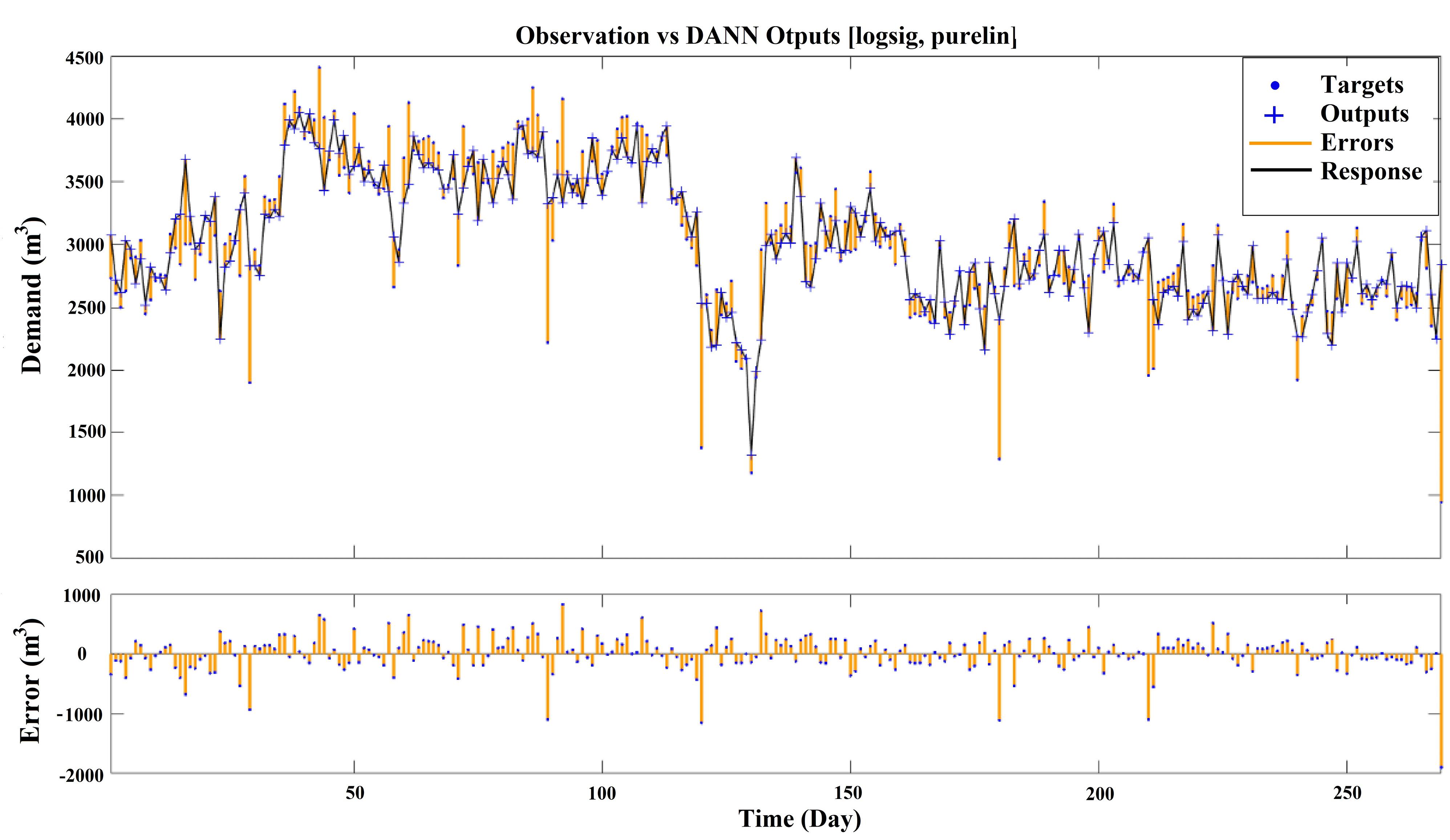
Fig. 8.
Observations vs. Best TANN Model Output with Sigmoidal Transfer Function in the Hidden Layer and Linear Transfer Function in the Output Layer
.
Observations vs. Best TANN Model Output with Sigmoidal Transfer Function in the Hidden Layer and Linear Transfer Function in the Output Layer
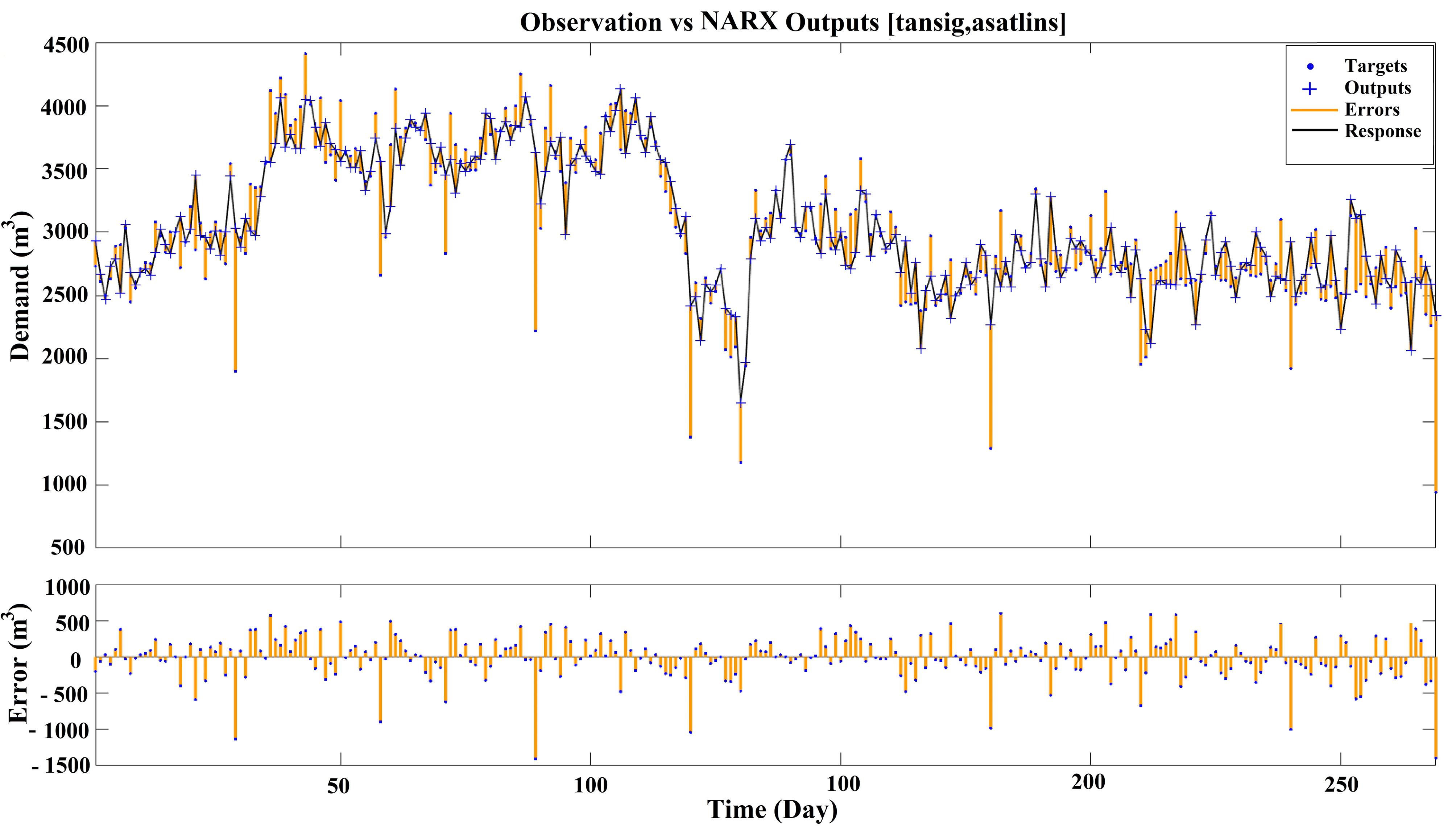
Fig. 9.
Observations vs. Best NARX Model Output with Hyperbolic Tangent Sigmoid Transfer Function in the Hidden Layer and Symmetric Saturating Linear Transfer Function in the Output Layer
.
Observations vs. Best NARX Model Output with Hyperbolic Tangent Sigmoid Transfer Function in the Hidden Layer and Symmetric Saturating Linear Transfer Function in the Output Layer
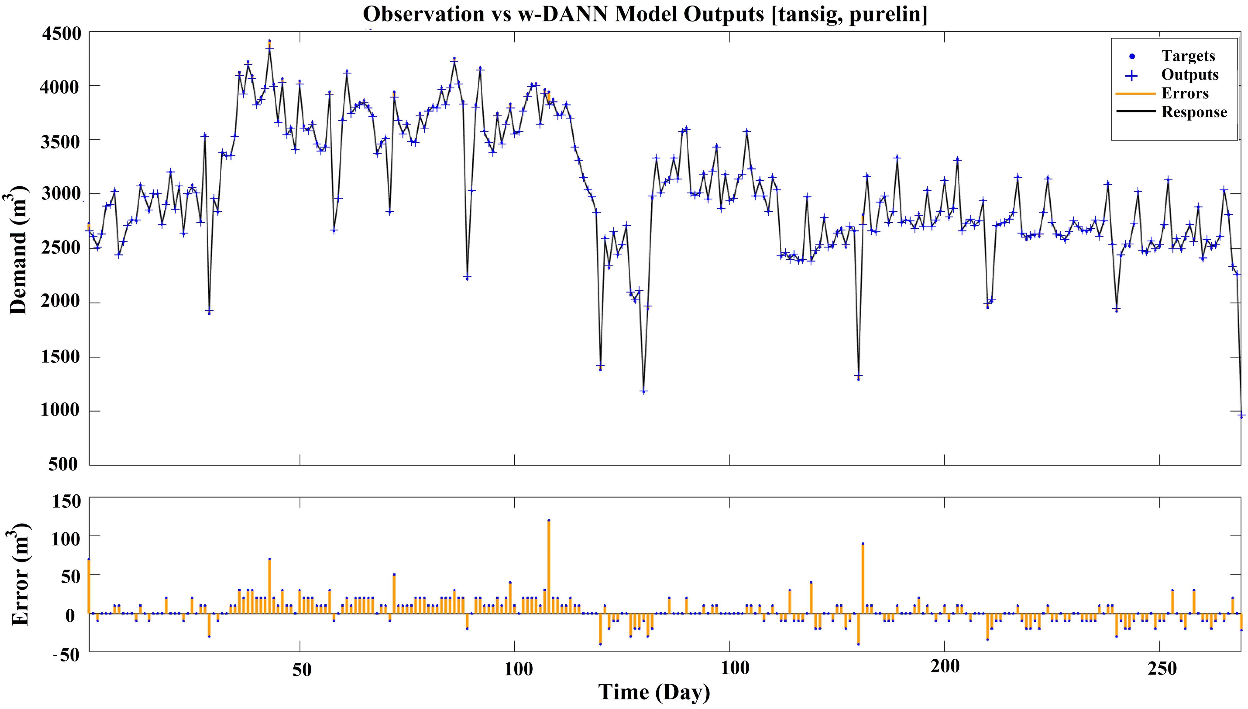
Fig. 10.
Observations vs. Best w-TANN Model Output with Hyperbolic Tangent Sigmoid Transfer Function in the Hidden Layer and Linear Transfer Function in the Output Layer
.
Observations vs. Best w-TANN Model Output with Hyperbolic Tangent Sigmoid Transfer Function in the Hidden Layer and Linear Transfer Function in the Output Layer
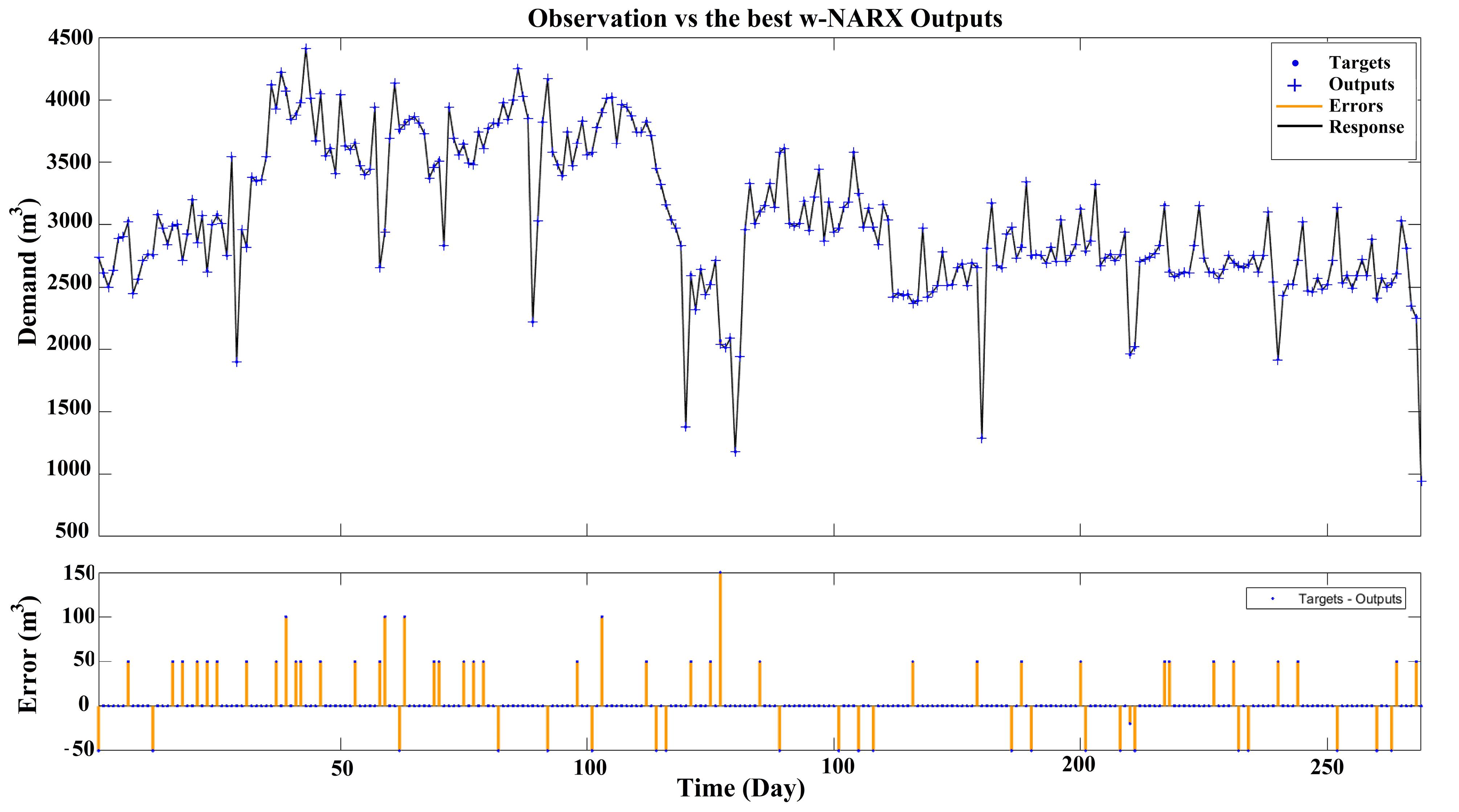
Fig. 11.
Observations vs. Best w-NARX Model Output with Hyperbolic Tangent Sigmoid Transfer Function in the Hidden Layer and Symmetric Saturating Linear Transfer Function in the Output Layer
.
Observations vs. Best w-NARX Model Output with Hyperbolic Tangent Sigmoid Transfer Function in the Hidden Layer and Symmetric Saturating Linear Transfer Function in the Output Layer
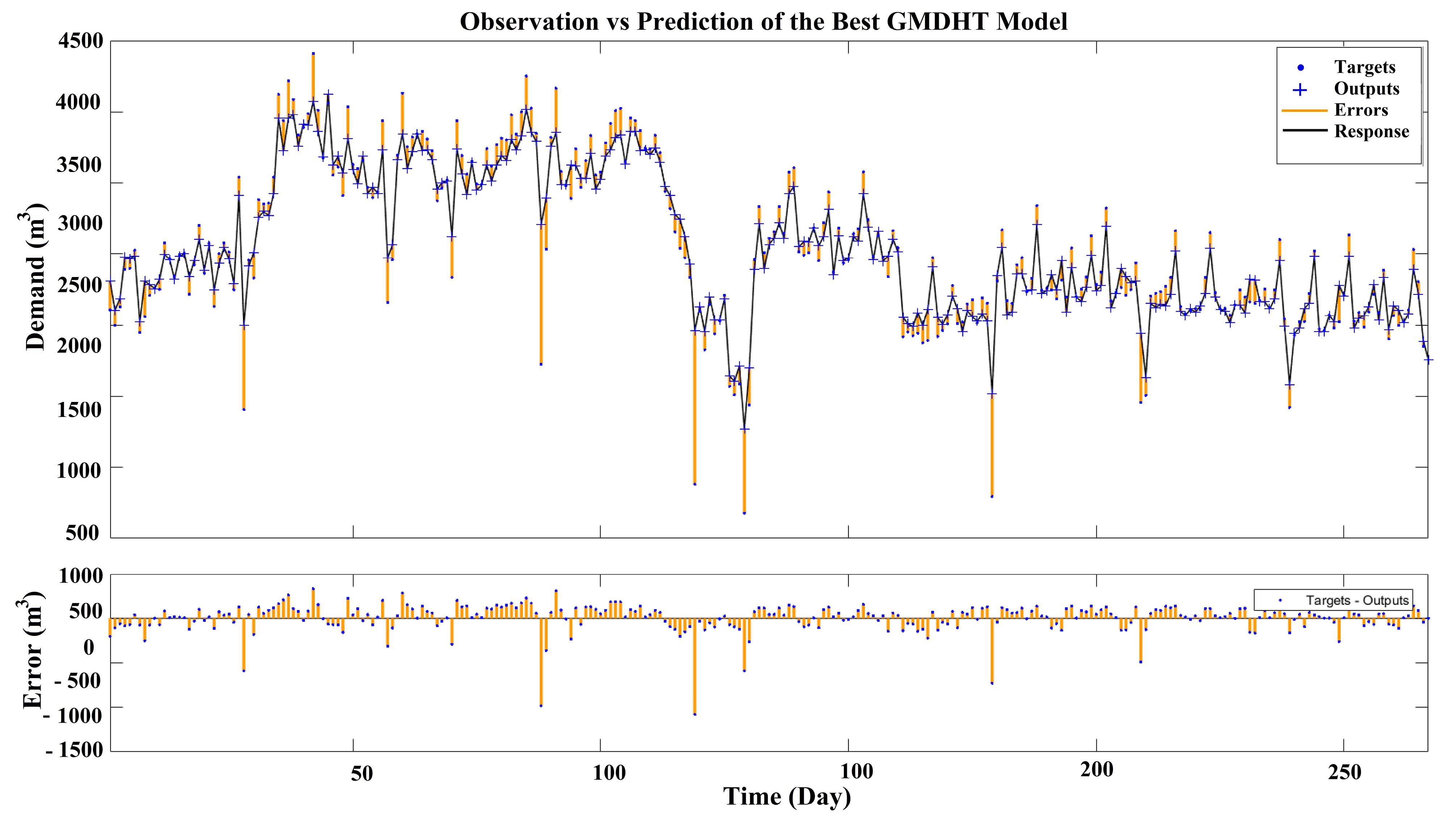
Fig. 12.
Observations vs. Prediction of the Best GMDHT Model Output with Five Neurons and Three Layers
.
Observations vs. Prediction of the Best GMDHT Model Output with Five Neurons and Three Layers
As is shown in these figures, the performance of w-TANN and w-NARX is better compared to others. The frequency of errors is much lower in w-NARX than in w-TANN. Comparing the TANN/w-TANN and NARX/w-NARX indicates that coupling WT with NARX networks is about two times more efficient in improving the performance of the networks than TANN. Additionally, the GMDHT model was found to be more accurate than both NARX and TANN. Based on this, GMDHT might be a good alternative when wavelet analysis is not preferred.
Utilizing NARX models (as an example of the best-performing model in this research) for predicting urban water demand offers a multitude of applications and advantages. These models facilitate precise demand forecasting by capturing intricate relationships between factors such as weather, population growth, and industrial activities. They enable real-time monitoring, enhancing the ability of water utilities to adapt to changing demand patterns. NARX models empower effective water resource management, support demand response programs, aid in leak detection, and assist in climate change adaptation (5,48). Additionally, they contribute to sustainability planning, optimize infrastructure investments, and promote data-driven decision-making, leading to energy savings and overall improved urban water system efficiency (2).
4. Conclusion
In this study, the potential of using WA in urban water demand prediction for ANN-based models, such as TANN, NARX, and GMDHT, is addressed. Among all of the mentioned models, TANN had the lowest performance in terms of MSE and RMSE. The most accurate method was found to be w-NARX. However, the results of the GMDHT method were also promising, especially when compared to TANN and NARX. NARX neural networks, when coupled with WT, were about two times better than TANN when coupled with WT.
The results of this research emphasize the fact that model structure plays an important role in model performance. The prominent examples of this role are the feedback connection in NARX models and the self-organizing principles of GMDH models, both of which are investigated in this study. This experimental comparison indicates that NARX neural networks can be considered as an alternative in future studies. The main advantage of NARX neural networks when compared to TANN is the feedback connection which may help to learn idiosyncrasies better than TANN.
Acknowledgments
The authors would like to appreciate Qom Water and Wastewater Company and Iran Meteorological Organization for providing data for this research. This study was approved by the Qom University of Medical Science (IR.MUQ.REC.1398.046, approval date: 2019-06-11).
Authors’ Contribution
Conceptualization: Reza Fouladi-Fard, Mostafa Rezaali, Abdolreza Karimi.
Data curation: Mostafa Rezaali, Reza Fouladi-Fard, Abdolreza Karimi.
Formal Analysis: Mostafa Rezaali, Abdolreza Karimi.
Funding acquisition: Reza Fouladi-Fard.
Investigation: Mostafa Rezaali, Abdolreza Karimi, Reza Fouladi-Fard.
Methodology: Mostafa Rezaali.
Project administration: Reza Fouladi-Fard, Abdolreza Karimi.
Resources: Reza Fouladi-Fard, Abdolreza Karimi.
Software: Mostafa Rezaali.
Supervision: Reza Fouladi-Fard, Abdolreza Karimi.
Validation: Mostafa Rezaali.
Visualization: Mostafa Rezaali.
Writing–original draft: Mostafa Rezaali.
Writing–review & editing: Reza Fouladi-Fard, Mostafa Rezaali, Abdolreza Karimi.
Competing Interests
The authors declare that they have no competing interests
Funding
This study received financial support from the Research Center for Environmental Pollutants, Qom University of Medical Sciences (grant number: 981011).
References
- Herrera M, Torgo L, Izquierdo J, Pérez-García R. Predictive models for forecasting hourly urban water demand. J Hydrol 2010; 387(1-2):141-50. doi: 10.1016/j.jhydrol.2010.04.005 [Crossref] [ Google Scholar]
- Rezaali M, Quilty J, Karimi A. Probabilistic urban water demand forecasting using wavelet-based machine learning models. J Hydrol 2021; 600:126358. doi: 10.1016/j.jhydrol.2021.126358 [Crossref] [ Google Scholar]
- Maier HR, Dandy GC. Neural networks for the prediction and forecasting of water resources variables: a review of modelling issues and applications. Environ Model Softw 2000; 15(1):101-24. doi: 10.1016/s1364-8152(99)00007-9 [Crossref] [ Google Scholar]
- Ghiassi M, Zimbra DK, Saidane H. Urban water demand forecasting with a dynamic artificial neural network model. J Water Resour Plan Manag 2008; 134(2):138-46. doi: 10.1061/(asce)0733-9496(2008)134:2(138) [Crossref] [ Google Scholar]
- Adamowski J, Karapataki C. Comparison of multivariate regression and artificial neural networks for peak urban water-demand forecasting: evaluation of different ANN learning algorithms. J Hydrol Eng 2010; 15(10):729-43. doi: 10.1061/(asce)he.1943-5584.0000245 [Crossref] [ Google Scholar]
- Mojarrad H, Fouladi Fard R, Rezaali M, Heidari H, Izanloo H, Mohammadbeigi A. Spatial trends, health risk assessment and ozone formation potential linked to BTEX. Hum Ecol Risk Assess 2020; 26(10):2836-57. doi: 10.1080/10807039.2019.1688640 [Crossref] [ Google Scholar]
- Fouladi Fard R, Naddafi K, Hassanvand MS, Khazaei M, Rahmani F. Trends of metals enrichment in deposited particulate matter at semi-arid area of Iran. Environ Sci Pollut Res 2018; 25(19):18737-51. doi: 10.1007/s11356-018-2033-z [Crossref] [ Google Scholar]
- Khazaei M, Mahvi AH, Fouladi Fard R, Izanloo H, Yavari Z, Tashayoei HR. Dental caries prevalence among schoolchildren in urban and rural areas of Qom province, central part of Iran. Middle East J Sci Res 2013; 18(5):584-91. doi: 10.5829/idosi.mejsr.2013.18.5.81155 [Crossref] [ Google Scholar]
- Fouladi Fard R, Hosseini MR, Faraji M, Omidi Oskoue A. Building characteristics and sick building syndrome among primary school students. Sri Lanka J Child Health 2018; 47(4):332-7. [ Google Scholar]
- Qom News. 2017. [Persian]. Available from: http://www.qomnews.ir/news/45162/%D8%AA%D8%A7%D9%85%DB%8C%D9%86-85-%D8%AF%D8%B1%D8%B5%D8%AF-%D8%A2%D8%A8-%D8%B4%D8%B1%D8%A8-%D8%B4%D9%87%D8%B1-%D9%82%D9%85-%D8%B3%D8%B1%D8%B4%D8%A7%D8%AE%D9%87-%D9%87%D8%A7%DB%8C-%D8%AF%D8%B2.
- Rezaali M, Karimi A, Moghadam Yekta N, Fouladi Fard R. Identification of temporal and spatial patterns of river water quality parameters using NLPCA and multivariate statistical techniques. Int J Environ Sci Technol 2020; 17(5):2977-94. doi: 10.1007/s13762-019-02572 [Crossref] [ Google Scholar]
- George EI. The variable selection problem. J Am Stat Assoc 2000; 95(452):1304-8. doi: 10.1080/01621459.2000.10474336 [Crossref] [ Google Scholar]
- Galelli S, Castelletti A. Tree‐based iterative input variable selection for hydrological modeling. Water Resour Res 2013; 49(7):4295-310. doi: 10.1002/wrcr.20339 [Crossref] [ Google Scholar]
- Hornik K, Stinchcombe M, White H. Multilayer feedforward networks are universal approximators. Neural Netw 1989; 2(5):359-66. doi: 10.1016/0893-6080(89)90020-8 [Crossref] [ Google Scholar]
- Govindaraju RS, Rao AR. Artificial Neural Networks in Hydrology. Springer Science & Business Media; 2013.
- Hansen JV, Nelson RD. Neural networks and traditional time series methods: a synergistic combination in state economic forecasts. IEEE Trans Neural Netw 1997; 8(4):863-73. doi: 10.1109/72.595884 [Crossref] [ Google Scholar]
- Pollock DS, Green RC, Nguyen T. Handbook of Time Series Analysis, Signal Processing, and Dynamics. Academic Press; 1999.
- Chan RWK, Yuen JKK, Lee EWM, Arashpour M. Application of nonlinear-autoregressive-exogenous model to predict the hysteretic behaviour of passive control systems. Eng Struct 2015; 85:1-10. doi: 10.1016/j.engstruct.2014.12.007 [Crossref] [ Google Scholar]
- Lin T, Horne BG, Tino P, Giles CL. Learning long-term dependencies in NARX recurrent neural networks. IEEE Trans Neural Netw 1996; 7(6):1329-38. doi: 10.1109/72.548162 [Crossref] [ Google Scholar]
- Xie H, Tang H, Liao YH. Time series prediction based on NARX neural networks: an advanced approach. In: 2009 International Conference on Machine Learning and Cybernetics. Hebei: IEEE; 2009. 10.1109/icmlc.2009.5212326.
- Alexandridis AK, Zapranis AD. Wavelet neural networks: a practical guide. Neural Netw 2013; 42:1-27. doi: 10.1016/j.neunet.2013.01.008 [Crossref] [ Google Scholar]
- Quilty J, Adamowski J. Addressing the incorrect usage of wavelet-based hydrological and water resources forecasting models for real-world applications with best practices and a new forecasting framework. J Hydrol 2018; 563:336-53. doi: 10.1016/j.jhydrol.2018.05.003 [Crossref] [ Google Scholar]
- Rezaali M, Fouladi Fard R, Mojarad H, Sorooshian A, Mahdinia M, Mirzaei N. A wavelet-based random forest approach for indoor BTEX spatiotemporal modeling and health risk assessment. Environ Sci Pollut Res 2021; 28(18):22522-35. doi: 10.1007/s11356-020-12298-3 [Crossref] [ Google Scholar]
- Ivakhnenko AG. Heuristic self-organization in problems of engineering cybernetics. Automatica 1970; 6(2):207-19. doi: 10.1016/0005-1098(70)90092-0 [Crossref] [ Google Scholar]
- Farlow SJ. The GMDH algorithm of Ivakhnenko. Am Stat 1981; 35(4):210-5. doi: 10.1080/00031305.1981.10479358 [Crossref] [ Google Scholar]
- Ivakhnenko AG. Polynomial theory of complex systems. IEEE Trans Syst Man Cybern 1971; SMC-1(4):364-78. doi: 10.1109/tsmc.1971.4308320 [Crossref] [ Google Scholar]
- Ivakhnenko AG, Ivakhnenko GA. The review of problems solvable by algorithms of the group method of data handling (GMDH). Pattern Recognition and Image Analysis 1995; 5(4):527-35. [ Google Scholar]
- Yarpiz. Group Method of Data Handling (GMDH) in MATLAB. 2018. Available from: http://yarpiz.com/263/ypml113-gmdh.
- Duerr I, Merrill HR, Wang C, Bai R, Boyer M, Dukes MD. Forecasting urban household water demand with statistical and machine learning methods using large space-time data: a comparative study. Environ Model Softw 2018; 102:29-38. doi: 10.1016/j.envsoft.2018.01.002 [Crossref] [ Google Scholar]
- Olden JD, Jackson DA. Illuminating the “black box”: a randomization approach for understanding variable contributions in artificial neural networks. Ecol Modell 2002; 154(1-2):135-50. doi: 10.1016/s0304-3800(02)00064-9 [Crossref] [ Google Scholar]
- Basheer IA, Hajmeer M. Artificial neural networks: fundamentals, computing, design, and application. J Microbiol Methods 2000; 43(1):3-31. doi: 10.1016/s0167-7012(00)00201-3 [Crossref] [ Google Scholar]
- Hagan MT, Menhaj MB. Training feedforward networks with the Marquardt algorithm. IEEE Trans Neural Netw 1994; 5(6):989-93. doi: 10.1109/72.329697 [Crossref] [ Google Scholar]
- Mukherjee I, Routroy S. Comparing the performance of neural networks developed by using Levenberg–Marquardt and Quasi-Newton with the gradient descent algorithm for modelling a multiple response grinding process. Expert Syst Appl 2012; 39(3):2397-407. doi: 10.1016/j.eswa.2011.08.087 [Crossref] [ Google Scholar]
- Kermani BG, Schiffman SS, Nagle HT. Performance of the Levenberg–Marquardt neural network training method in electronic nose applications. Sens Actuators B Chem 2005; 110(1):13-22. doi: 10.1016/j.snb.2005.01.008 [Crossref] [ Google Scholar]
- Cigizoglu HK, Kişi Ö. Flow prediction by three back propagation techniques using K-fold partitioning of neural network training data. Hydrol Res 2005; 36(1):49-64. [ Google Scholar]
- Yarpiz. Time-Series Prediction using GMDH in MATLAB MATLAB Central File Exchange. 2015. Available from: https://www.mathworks.com/matlabcentral/fileexchange/52972-time-series-prediction-using-gmdh-in-matlab.
- Joo CN, Koo JY, Yu MJ. Application of short-term water demand prediction model to Seoul. Water Sci Technol 2002; 46(6-7):255-61. doi: 10.2166/wst.2002.0687 [Crossref] [ Google Scholar]
- Firat M, Turan ME, Yurdusev MA. Comparative analysis of fuzzy inference systems for water consumption time series prediction. J Hydrol 2009; 374(3-4):235-41. doi: 10.1016/j.jhydrol.2009.06.013 [Crossref] [ Google Scholar]
- Wu CL, Chau KW, Li YS. Predicting monthly streamflow using data-driven models coupled with data-preprocessing techniques. Water Resour Res 2009; 45(8):1-23. doi: 10.1029/2007wr006737 [Crossref] [ Google Scholar]
- Uddameri V, Singaraju S, Hernandez EA. Is standardized precipitation index (SPI) a useful indicator to forecast groundwater droughts?—Insights from a karst aquifer. J Am Water Resour Assoc 2019; 55(1):70-88. [ Google Scholar]
- Alhamshry A, Fenta AA, Yasuda H, Shimizu K, Kawai T. Prediction of summer rainfall over the source region of the Blue Nile by using teleconnections based on sea surface temperatures. Theor Appl Climatol 2019; 137(3):3077-87. doi: 10.1007/s00704-019-02796-x [Crossref] [ Google Scholar]
- Cebrián AC, Abaurrea J, Asín J, Segarra E. Dynamic regression model for hourly river level forecasting under risk situations: an application to the Ebro river. Water Resour Manag 2019; 33(2):523-37. doi: 10.1007/s11269-018-2114-2 [Crossref] [ Google Scholar]
- Rajaee T, Ravansalar M, Adamowski JF, Deo RC. A new approach to predict daily pH in rivers based on the “à trous” redundant wavelet transform algorithm. Water Air Soil Pollut 2018; 229(3):85. doi: 10.1007/s11270-018-3715-3 [Crossref] [ Google Scholar]
- Prasad R, Deo RC, Li Y, Maraseni T. Input selection and performance optimization of ANN-based streamflow forecasts in the drought-prone Murray Darling Basin region using IIS and MODWT algorithm. Atmos Res 2017; 197:42-63. doi: 10.1016/j.atmosres.2017.06.014 [Crossref] [ Google Scholar]
- Heidari E, Daeichian A, Sobati MA, Movahedirad S. Prediction of the droplet spreading dynamics on a solid substrate at irregular sampling intervals: Nonlinear Auto-Regressive eXogenous Artificial Neural Network approach (NARX-ANN). Chem Eng Res Des 2020; 156:263-72. doi: 10.1016/j.cherd.2020.01.033 [Crossref] [ Google Scholar]
- Bata MT, Carriveau R, Ting DS. Short-term water demand forecasting using nonlinear autoregressive artificial neural networks. J Water Resour Plan Manag 2020; 146(3):04020008. doi: 10.1061/(asce)wr.1943-5452.0001165 [Crossref] [ Google Scholar]
- Ebtehaj I, Bonakdari H, Zaji AH, Azimi H, Khoshbin F. GMDH-type neural network approach for modeling the discharge coefficient of rectangular sharp-crested side weirs. Eng Sci Technol Int J 2015; 18(4):746-57. doi: 10.1016/j.jestch.2015.04.012 [Crossref] [ Google Scholar]
- Adamowski J, Fung Chan H, Prasher SO, Ozga-Zielinski B, Sliusarieva A. Comparison of multiple linear and nonlinear regression, autoregressive integrated moving average, artificial neural network, and wavelet artificial neural network methods for urban water demand forecasting in Montreal, Canada. Water Resour Res 2012; 48(1):1-14. doi: 10.1029/2010wr009945 [Crossref] [ Google Scholar]