Avicenna J Environ Health Eng. 9(2):75-84.
doi: 10.34172/ajehe.2022.4206
Original Article
The Performance of Several Current Interpolation Methods for Variability of cations in Groundwater in Esfarayen Plain, Iran: A Case Study
Ali Mahmoodnia 1, Morteza Mousavi 2, Farshad Golbabaei Kootenaei 1, *  , Mahdi Asadi-Ghalhari 3
Author information:
1Department of Environmental Engineering, Faculty of Environment, Campus of Engineering, University of Tehran, Tehran, Iran
2Department of Environmental Engineering, Faculty of Civil Engineering, Khajeh Nasir University of Technology, Tehran, Iran
3Department of Environmental Health Engineering, Faculty of Health, Qom University of Medical Sciences, Qom, Iran
Abstract
Acquiring information about groundwater quality is essential in developing management strategies. In this article, spatio-temporal variations of cations in groundwater in Esfarayen plain were investigated using data monitored in 134 groundwater wells, active in 1988, and 47 wells, active in 2019. To evaluate groundwater quality, interpolation methods have been used to interpolate existing limited spatial data. The performance of 8 current interpolation methods on the data for the two selected years (1988 and 2019) was compared. Finding the optimum interpolation method for the considered groundwater quality parameters is essential. Cross-validation and three indexes of R2, mean absolute error (MAE), and root mean square error (RMSE) were used to compare the performance of the methods. By identifying universal kriging (UK) and global polynomial interpolation (GPI) methods as the optimum methods and using those for the selected years (1988 and 2019), spatial variation of the concentration of cations in groundwater across the plain has been presented. In 1988, the maximum concentration of the cations occurred in the southwest of the plain (about 80 mg/L), and the minimum concentration of the cations was observed in the northwest of the plain (approximately 8 mg/L). Similarly, in 2019, the highest concentration of the cations was found in the southwest of the plain (almost 64 mg/L), and its lowest concentration was observed in the northeast of the plain (roughly 13 mg/L). Moreover, temporal variations of the concentration of cations in groundwater from 1988 to 2019 have also been presented. The concentration of the cations increased by approximately 23 mg/L in the northwest and decreased to about 37 mg/L in the southwest of the study area from 1988 through 2019. According to the results, changes in the quality of groundwater are a complex problem and it is necessary to adopt proper strategies to reduce its adverse effects.
Keywords: Groundwater, Cation, Interpolation methods, Spatio-temporal variability,
Copyright and License Information
© 2022 The Author(s); Published by Hamadan University of Medical Sciences.
This is an open-access article distributed under the terms of the Creative Commons Attribution License (
http://creativecommons.org/licenses/by/4.0), which permits unrestricted use, distribution, and reproduction in any medium provided the original work is properly cited.
Please cite this article as follows: Mahmoodnia A, Mousavi M, Golbabaei Kootenaei F, Asadi-Ghalhari M. The performance of several current interpolation methods for variability of cations in groundwater in Esfarayen plain, Iran: a case study. Avicenna J Environ Health Eng. 2022; 9(2):75-84. doi:10.34172/ajehe.2022.4206
1. Introduction
Water is known as one of the most crucial and abundant resources on the planet (1). Water covers about three-quarters of the earth’s surface. However, out of the total water available on the planet, about 97% is salt water and less than 3% is freshwater. Less than 1% of Earth’s water is freshwater that is directly available to humans, while two-thirds or more of it is frozen in polar regions. The remaining unfrozen freshwater is mainly known as groundwater, with a small portion as surface water and atmospheric water (2). The rapid increase in population, the advancements in developing countries, and the mismanagement of water resources have caused a considerable increase in water use, leading to a warning of water shortage worldwide. Therefore, despite the technological progress of the present modern era, water-related issues persist as a daunting challenge of the 21st century (3).
In the recent century, global water demand has incremented at more than twice the population growth rate (4). In these circumstances, water shortage is one of the most critical limitations of life, affecting domestic, industrial, and agricultural issues (5). According to a scenario, the globe will face about 40% water shortage and/or supply-demand gap by 2030 (6).
Among the various sources of water on earth, groundwater is of great importance. Groundwater is acknowledged as the primary precious natural water resource for irrigation, industrial and drinking water in many areas, especially in arid regions (7-9). Irrigation with poor-quality water can change the physicochemical properties of the soil, reducing crop productivity and causing soil salinization (10,11). Currently, the reliable water resource has changed into an essential resource of the globe (12). It is reported that about 2.5 billion individuals worldwide rely on groundwater to satisfy their needs for drinking water (13).
Groundwater could be used cheaper and more effortlessly in underdeveloped countries. Moreover, groundwater has been even the only dependable water resource in many regions around the world. For example, Iran is known as an arid and semi-arid part of the earth (14). Groundwater is the main water resource for about 50% of individuals living in Iran’s urban areas and 70% or more of Iranians that live in rural areas (15). This led to groundwater withdrawal in many areas in Iran, which in turn caused very harmful consequences (16).
The most critical consequences of groundwater overuse in tens of countries globally, including Iran, include land subsidence, saltwater intrusion into coastal aquifers, damage to ecosystems, and pollution of water resources (17). Therefore, it is essential to evaluate groundwater quality, especially in areas with a deep water table and regions with an extremely high water table, in which the soil that may suffer from some problems such as salinity and waterlogging (18).
Evaluating groundwater quality needs interpolating the existing spatially distributed data, which is limited because sampling and mapping are complicated in Earth science. Geostatistics provides a valuable tool to handle spatially distributed data, including groundwater and soil pollution (18). In recent years, many scientists have compared different interpolation methods in various situations, and geographical information system (GIS) has been a powerful tool for analyzing groundwater quality. Additionally, some reports have compared the performance of other interpolation methods in estimating groundwater depth in arid regions (19-21). Moreover, Due to the health effects of some cations in the water (sodium, calcium, magnesium, potassium), the researcher focused on different aspects of these cations (22,23). Ramyapriya and Elgano found that based on the concentration of major ions, most of the groundwater samples were unsuitable for drinking purposes along the Cauvery River (24). Similarly, research demonstrates that due to the existence of ions such as magnesium (Mg) in the groundwater within the urban reach of Gridhumal river, groundwater is unsuitable for either drinking or irrigation purposes (25).
To our knowledge, there is no study investigating the concentration of cations in groundwater in Esfarayen plain. Therefore, the present work aimed to investigate the spatial and temporal variations of the cation concentration during 1988-2019 in Esfarayen plain. Multivariate statistical analysis and GIS-based thematic maps were used to investigate Spatio-temporal changes in the concentration of cation in the groundwater. In this way, the optimal interpolation method was selected among inverse distance weighting (IDW), radial basis function (RBF), GPI, local polynomial interpolation (LPI), universal kriging (UK), ordinary kriging (OK), simple kriging (SK), and diffusion kernel (DK) methods to investigate cation concentration in Esfarayen plain. The accuracy of the estimations from those methods was compared, and the error values were analyzed. Secondly, the most efficient method was used to provide the Spatio-temporal variabilities of cation concentration in the groundwater of Esfarayen plain.
2. Materials and Methods
2.1. Study Area
Esfarayen plain is a part of Iran’s central desert located in the south of the Northern Khorasan province of Iran (Fig. 1). Esfarayen plain has a semi-arid climate with almost cold winters and moderate summers. Like other arid and semi-arid plains of Iran, groundwater resources in this plain are vital for agricultural purposes, domestic use, and industrial activities (26). The number of wells and coordinates of points is demonstrated in Tables S1 and S2 (See Supplementary file 1).
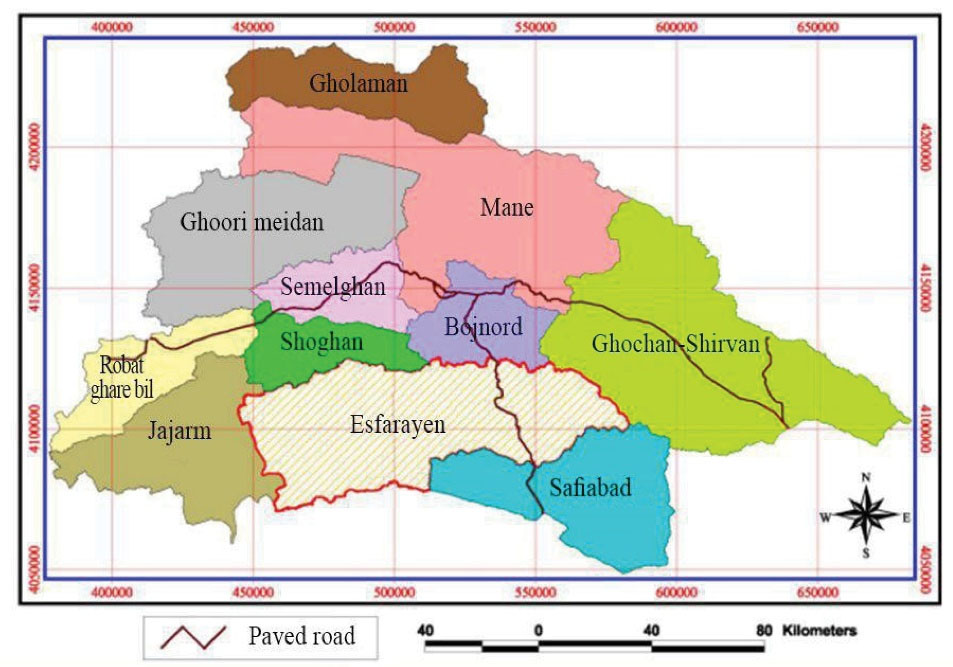
Fig. 1.
The Location of the Study Area.
.
The Location of the Study Area.
2.2. Interpolation Methods
The current work is categorized as a quantitative study that addresses the spatial and temporal variations of cation concentration in the groundwater of Esfarayen plain. Statistical analyses were carried out using MINITAB software version 18. The existing data were not normal in any of the selected years, considering the values of Skew and Kurtosis shown in Table 1. According to Table 1, in the year 1988, positive skewness of 2.89 indicates the bias in distributing data toward the right. A positive kurtosis of 11.64 implies the sharpness of data distribution and shows the closeness of the data to the average amount. Moreover, in the year 2019, the positive skewness of 1.011 shows the bias in the distribution of the data toward the right; however, the negative kurtosis of -0.145 shows that the data are far from the average amount. For data normalization, the logarithmic transformation was applied using MINITAB software.
Table 1.
Statistical Analysis of Groundwater Cations
|
Year
|
No.
|
Min
|
Max
|
Med
|
Mean
|
Skew
|
SD
|
Kurtosis
|
Range
|
| 1988 |
135 |
6.3 |
205 |
20.3 |
30.3 |
2.89 |
28.58 |
11.64 |
198.7 |
| 2019 |
47 |
7.1 |
65.5 |
17.2 |
25.37 |
1.011 |
18.13 |
-0.145 |
58.4 |
After normalizing the data, the interpolation methods of IDW, RBF, GPI, LPI, UK, OK, SK, and DK were applied. Normalizing the data was needed only for Kriging methods (DK, SK, and OK) (27). Finally, after the comparison of the results, the optimum method was selected and used for providing the Spatio-temporal variations of concentration of groundwater cations, including potassium (K), sodium (Na), magnesium (Mg), and calcium (Ca) in Esfarayen plain. Fig. 2 shows the flowchart used for the interpolations.
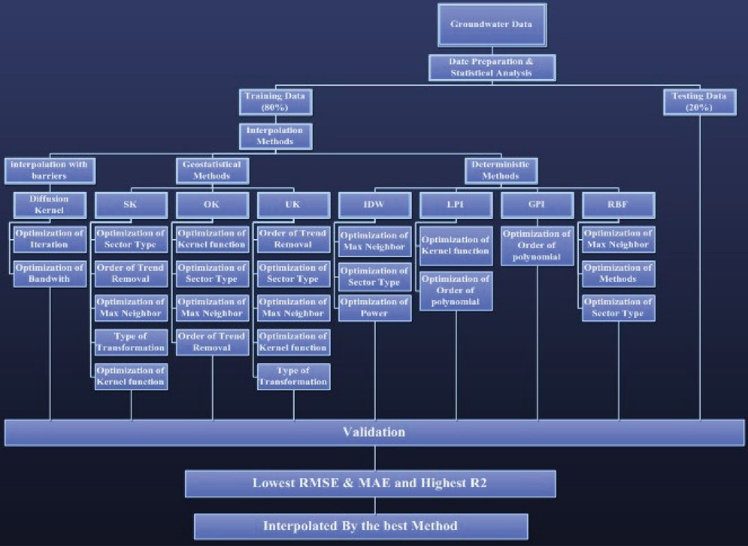
Fig. 2.
Flowchart of Interpolation Methods and Selection of the Best Method in Estimating Groundwater Cation.
.
Flowchart of Interpolation Methods and Selection of the Best Method in Estimating Groundwater Cation.
2.2.1. Inverse Distance Weighting Method
The IDW calculates the quantity of a parameter at the points of interest. This method is recognized as one of the well-known interpolation methods (28). The process uses a linear combination of values at sampled points weighted by an inverse function of the distances between the sampled points and the points of interest (29). IDW is often used in GIS for creating raster overlays from data points. If the data were on a regular grid, contour lines could be threaded across the interpolated values, and the map could be prepared either as a raster-shaded or vector contour map (10). The values are estimated using equation 1 as below (30).
(1)
where
Z: the estimated value
Zi: the measured sample value at a point
di: the distance between Z and Zi
m: the weighting power
It should be noted that if m is described as the rate that weights fall off with di, the m value commonly varies from 1 to 5. In this study, the estimates of IDW were compared using typical weighting powers (including 1, 2, 3, 4, and 5). Meanwhile, m was set to 1 for both of the selected years (27).
2.2.2. Radial Basis Function
RBF methods are a series of exact interpolation techniques in which the surface must pass through all measured values (27). RBF values depend only on the distance from the origin and/or the distance from another point called a center (31). There are five different basis functions: thin-plate spline, spline with tension, completely regularized spline, multiquadric function, and inverse multiquadric function (IMQ) (10). This study used IMQ for both years (1988 and 2019).
2.2.3. Kriging Method
Kriging is a regression method known as a partial spatial interpolation method (32). Kriging is recognized as the best linear unbiased technique for estimating the value of regionalized variables at unsampled locations (27). It is based on the accessible data of regionalized variables and structural characteristics of a variogram. It can be classified into OK, UK, and SK.
The estimator of SK is Equation 2 (30).
where
n: the number of values used for estimation
m: the mean value
: the estimated value at x0
Z(Xi): the measured value at Xi
λi: the weight assigned to the residual of Z(Xi); their summation is 1 (33)
The estimator of OK is given by (30):
where the variables definition of equation 3 is as equation 2.
The UK has been known as a geostatistical technique for a linear unbiased estimator, considering the deterministic component. The covariance’s column vector for non-statistic random function and variogram is given below (30). Therefore, the expected value of Z(X) at point Z is m(x) (by definition of the drift component):
The interpolation expressions take the form of:
where
n: the number of available sampling data
: the estimated value
Zα: the measured value at sampling point α (α = 1... n)
λα: the weighting coefficient, calculated with the unbiased and minimum error variance
The UK was the best method for the first selected year (1988); however, SK had the optimized performance for the second year chosen (2019).
2.2.4. Global Polynomial Interpolation
Global polynomial interpolation (GPI) fits a smooth surface that is well defined by a mathematical function to the input sample points (34). The surface of GPI has gradual changes and catches coarse-scale patterns in the data (29). GPI has a smoothly varying surface using low-order polynomials, which possibly depict some physical processes. However, the more complex the polynomial, the more difficult it is to ascribe physical meaning to it. Further, the measured surface is considered susceptible to outliers (extraordinarily low and high values), mainly at the edges (30). A first-order global polynomial fits a single plane passing through the data; a second-order GP fits a surface with a bend in it, allowing the surfaces representing valleys; a third-order GP allows for two bends; and so forth. However, when a surface has a different shape, a single GP will not fit it well (30).
2.2.5. Local Polynomial Interpolation
Unlike GPI, which fits a polynomial to the whole surface, LPI fits numerous polynomials within a defined overlapping neighborhood (35). The search neighborhood can be described utilizing the search neighborhood dialog. The shape, minimum and maximum numbers of points, and sector arrangement can be specified. Alternatively, a slider can be used to define the width of the neighborhood in conjunction with a power parameter. The power variable will diminish the weights of the sample points within the neighborhood based on distance. Hence, LPI provides surfaces that account for more local changes (30).
2.2.6 Diffusion Kernel
Diffusion Interpolation refers to the fundamental solution of the heat equation, which describes how heat or particles diffuse with time in a homogeneous medium. Diffusion interpolation produces predictions on automatically selected grids (cells), while all other models in geostatistical analysis use triangles of various sizes (36).
2.2.7. Optimum Interpolation Methods
Validation and cross-validation help the decision-making process to find out which technique gives the most reliable predictions. Many scientists have applied different training and testing sets to determine the most reliable method. They also used various comparison approaches to find the relationships between observed and predicted values and subsequently determine the best technique (10). In this study, the groundwater wells were divided into two groups randomly; in other words, 80 % of the sampling points were applied to develop the model, and 20% were used for an independent validation process. Three statistical indexes of mean absolute error (MAE), root mean square error (RMSE), and R2 were utilized to investigate interpolation methods. The lowest RMSE and MAE and the highest R2 indicate the most precise predictions. Estimates are defined by applying the following equations (30,37):
(8)
Where;
Zi: the predicted value
Z: the observed value
N: the number of observations
3. Results and Discussion
Detailed statistics on groundwater cation measures for the selected years (1988 and 2019) are presented in Table 1.
The groundwater cation concentration varied between 6.3 and 205 mg/L in 1988 and between 7.1 and 65.5 mg/L in 2019.
Stochastic techniques are ordinarily reliable if the data have a normal distribution. Therefore, the data should be checked in advance for a normal distribution. According to Kolmogorov–Smirnov test, data of groundwater cations during the two selected years were not normally distributed. Accordingly, values were log-transformed prior to semivariance estimation. Their influential parameters should be determined to optimize the results of the interpolation methods.
In IDW method, each power, max neighbors, and sector type factor should be optimized. At first, the power should be optimized, and after optimizing the max neighbors and sector type, the power should be optimized again. The results of optimizing max neighbors and sector type for both selected years are illustrated in Table 2. As it is illustrated in Table 2, the IDW with 19 max neighbors, 4-4D type sector, and 1 as the power was optimized in 1988. Moreover, in 2019, the IDW with seven max neighbors, 1 type sector, and power of 1 was optimized.
Table 2.
The Summary of Validation Results for Cations in the Years 1988 and 2019
|
Interpolation Methods
|
Optimized Parameters
|
RMSE
|
MAE
|
|
|
1988
|
2019
|
1988
|
2019
|
1988
|
2019
|
| IDW |
Power |
1 |
1 |
20.45 |
19.74 |
5.7 |
-7.71 |
| Max neighbors |
19 |
7 |
| Sectors |
4-4D |
1 |
| Diffusion equation |
Bandwidth |
11000 |
4000 |
17.19 |
21.22 |
26.4 |
-8.89 |
| Iteration |
250 |
150 |
| Global polynomial |
Order of polynomial |
1 |
1 |
18.49 |
17.42 |
2.71 |
-11.05 |
| Local polynomial |
Order of polynomial |
1 |
3 |
18.75 |
20.57 |
4.51 |
-9 |
| Kernel function |
constant |
Exponential |
| RBF |
Method |
Inverse multiquadric function |
Inverse multiquadric function |
19.81 |
20.67 |
5.52 |
-8.98 |
| Max neighbors |
15 |
7 |
| Sector |
4-4D |
4-4D |
| Kriging |
method |
UK |
SK |
16.39 |
19.28 |
-0.497 |
-10.68 |
| Transformation |
Log |
Log |
| Trend removal |
constant |
First |
| Kernel function |
Polynomial |
Exponential |
| Max neighbors |
5 |
5 |
| Sector |
4 |
1 |
Abbreviations: IDW, inverse distance weighting; RBF, radial basis function; MAE, mean absolute error; RMSE, root mean square error.
RBF has 5 sub-functions, and all of them were used in the present study. The results of optimizing sub-functions and influential parameters of RBF for 1988 and 2019 are also presented in Table 2. In both of these selected years, RBF with sub-function of inverse multiquadric function yielded the best results.
In the present study, three versions of kriging, i.e., SK, OK, and UK, were used in both of the selected years (1988 and 2019). Essential characteristics and parameters of each version that must be considered are transformation type, the order of trend removal, kernel function, max neighbors, and sector type. The results of selecting the best version of kriging are presented in Table 2. As illustrated in Table 2, UK was the best version in 1988 and SK was selected as the best version in 2019.
In optimizing diffusion interpolation, the optimization of two parameters should be considered. The parameters are the number of iterations in the solution of the heat equation and bandwidth. The implementation of this method needs more time than IDW because time is heavily dependent on the number of iterations in the heat equation solution. Hence, first, bandwidth was optimized while the iteration number was 100. Secondly, the iteration number was optimized. Optimizing iteration numbers was not like optimizing the power of IDW; there is an oscillation between good and bad results. Table 2 shows the results of optimization of diffusion interpolation for 1988 and 2019.
The most crucial optimizing parameter in the GPI method is the polynomial order. The results of optimizing this parameter are also presented in Table 2. Order 1 for GPI yielded the best results for both selected years (1988 and 2019).
LPI has two critical parameters that should be optimized: the kernel function and the polynomial order. The order of polynomials was optimized as presented in Table 2. The best orders were 1 and 3 for 1988 and 2019, respectively. Kernel function was optimized for both of the selected years. In 1988, the constant kernel function was the best, but in 2019, the exponential kernel function yielded the best results.
As discussed, the validation result for groundwater cations in 1988 and 2019 was summarized in Table 2. This table consists of all the used methods, the best-fitted parameters for the methods, and finally, RMSE and MAE for each year. As it was previously mentioned, the best-fitted IDW had the power of 1, maximum neighbor of 19, and sector type of 4-4D for the year 1988.
For the DK, the bandwidth was 11 000, with the iteration number of 250 in the heat equation solution. Additionally, GPI with the order of 1 yielded the best result comparing the polynomial orders. Meanwhile, LPI with the order of 1 and constant kernel function was the best choice among different kinds of LPI, and the best-fitted RBF was IMQ with max neighbor of 15 and sector type of 4-4D. The best choices were the UK with log transformation with constant order of trend removal and a polynomial with kernel function with maximum neighbors of 5 and sector type of 4.
In 2019, the best-fitted IDW had power 1, and the maximum neighbors were 7; the sector type was 1. The best-fitted DK bandwidth was 4000. The iteration number was 150 in the solution of the heat equation. Additionally, GPI with the order of 1 yielded the best result compared to other polynomial orders. Meanwhile, LPI with the order of 1 and constant kernel function was the best choice among LPI kinds. The best-fitted RBF was IMQ with a maximum neighbor of 15 and sector type of 4-4D. Moreover, the UK with log transformation with constant order of trend removal was the optimum. Polynomial kernel function with maximum neighbor of 5 and sector type of 4 was the best choice.
As Fig. 3 shows, the UK technique with the optimized parameters showed a better correlation between the simulated and measured amounts in 1988. As Fig. 4 shows, the results from the GPI method with optimized parameters had a better correlation with the measured amounts of cations in 2019.
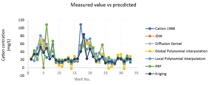
Fig. 3.
Correlation Analysis for Cations in 1988.
.
Correlation Analysis for Cations in 1988.
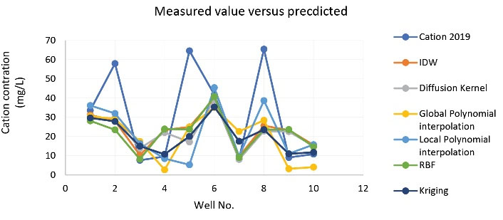
Fig. 4.
Correlation Analysis for Cations in 2019.
.
Correlation Analysis for Cations in 2019.
Considering Tables 2 and 3, in 1988, the UK method with the optimized parameters had both the least prediction error and the highest correlation with the measured amounts. Therefore, it is the best interpolation method for investigating spatial variations of cations in groundwater. As for the year 2019, the GPI method is the best interpolation method.
Table 3.
The Summary of Cross-validation Results for Cations in 1988 and 2019
|
Measurement of Error
|
IDW
|
DK
|
GPI
|
LPI
|
RBF
|
Kriging
|
| R (1988) |
0.551 |
0.539 |
0.59 |
0.59 |
0.519 |
0.625 |
| R2 (1988) |
0.303 |
0.29 |
0.348 |
0.348 |
0.267 |
0.391 |
| R (2019) |
0.768 |
0.668 |
0.841 |
0.707 |
0.705 |
0.809 |
| R2 (2019) |
0.59 |
0.446 |
0.708 |
0.499 |
0.497 |
0.654 |
Abbreviations: IDW, inverse distance weighting; DK, diffusion kernel; GPI, global polynomial interpolation; LPI, local polynomial interpolation; RBF, radial basis function.
Fig. 5 shows the spatial changes in the concentration of cations in Esfarayen plain in the year 1988 with the UK. Fig. 5 indicates that the highest cation concentration was observed in the southwest of the plain, decreasing toward the north in 1988.
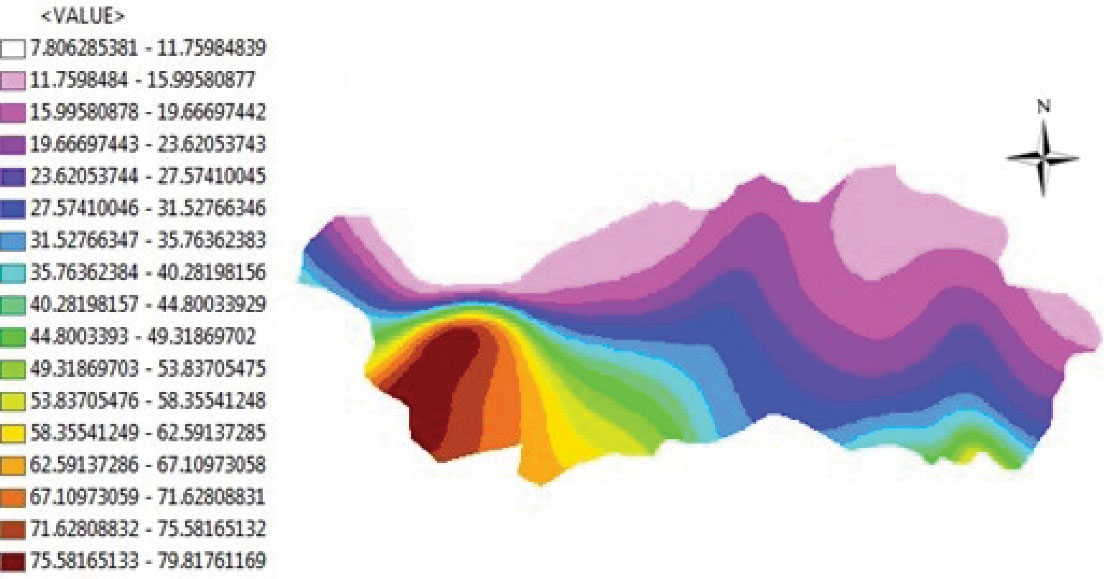
Fig. 5.
The Spatial Changes in the concentration of Cations in Esfarayen Plain in the Year 1988.
.
The Spatial Changes in the concentration of Cations in Esfarayen Plain in the Year 1988.
Fig. 6 shows the spatial variation of cation concentration in Esfarayen plain in 2019. Fig. 6 indicates that the highest concentration of cations was observed in the southwest of the plain in 2019, decreasing toward the northeast.
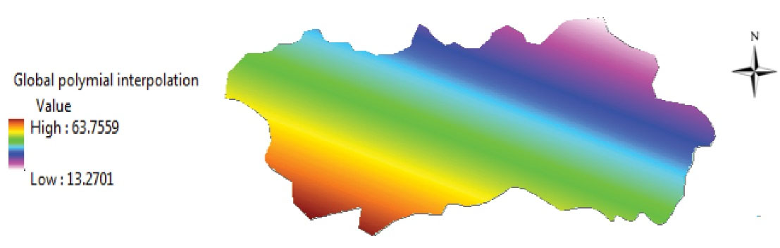
Fig. 6.
The Spatial Changes in the concentration of Cations in Esfarayen Plain in the Year 2019.
.
The Spatial Changes in the concentration of Cations in Esfarayen Plain in the Year 2019.
Fig. 7 presents the trend of the variation of cation concentration from the year 1988 to the year 2019. As Fig. 7 shows, the highest increase in the amount of cations was observed in the northwest, and the highest decrease in the amount of cations was found in the southeast from 1988 to 2019.
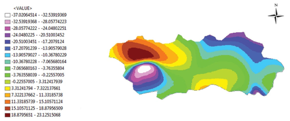
Fig. 7.
The Trend of the Variation of Cation Concentration from the Year 1988 to the Year 2019.
.
The Trend of the Variation of Cation Concentration from the Year 1988 to the Year 2019.
The results showed that the highest increase in the concentration of total cations has occurred in the northwest of the plain, primarily due to alluvial evaporation deposits that lead to an increment in the concentrations of Cl, Mg, and K. Moreover, considerable consumption of fertilizers containing Na, Ca, Mg, and K in the northwest of the plain for agricultural purposes is another reason for increasing the concentration of total cations in the northwest of the plain. Further, in a small part in the east of the plain, the concentration of cations decreased, mostly due to freshening in the aquifer due to rainfall and fresh ground discharge as well as ion adsorption during ion exchange. It was noted in similar studies that changes in the concentration of cations in the groundwater are mainly attributed to alluvial evaporation, extensive use of fertilizers, and ground discharge (38-40). The final maps of spatial changes of cations in the selected years are presented in Figs. 5 and 6. The optimization results showed that for 1988, the optimal interpolation method was UK (27), and for 2019, the optimal interpolation method was GPI (27). According to both maps, most of cation’s gloom occurred in the southwest of the plain and decreased to the northeast. The difference is that the maximum concentration in 2019 was lower than in 1988, which can be clearly seen in Fig. 7. The highest decrease in cation concentration was observed during the study period in the southeastern regions of the plain. In general, groundwater quality change is a complex problem (not a complicated one) occurring in many areas. One of the main reasons for this is the small changes in groundwater levels, and researchers and decision-makers must control the dimensions of this growing phenomenon by adopting appropriate policies and strategies (41,42).
GIS-based interpolation methods have widely been used in scientific research (43-46). For instance, Hazbavi and Gherachorlo (27) examined the performance of RBF, IDW, and Kriging-based interpolation methods for spatial and temporal groundwater level changes in Meshgin plain. They found that the RBF method with the lowest error is the optimum method for preparing the spatio-temporal map. Furthermore, Leulmi et al (47) evaluated the Spatio-temporal variation of nitrate (during 2006-2016) in groundwater in the Eastern Mitidja plain in Algeria. They used a geostatistical approach for drawing kriging maps for the nitrate level in the Mitidja plain. They asserted that nitrate fluctuation in the Mitidja plain was higher than WHO standards (higher than 50 mg/L). They explained these changes by anthropogenic factors and piezometric level changes. Similarly, Meng et al (37) compared the interpolation performance of seven GIS interpolation methods and cited that regression kriging can significantly improve spatial prediction accuracy even when using a weakly correlated auxiliary variable. Further, Adhikary and Dash (31) compared the performance of deterministic (IDW and RBF) and stochastic (UK and OK) methods to predict the spatial variation of groundwater depth in India. Their analysis revealed that the UK has the best performance in predicting the spatial variation of groundwater depth in India.
4. Conclusion
This study assessed spatio-temporal variation of the cations in the groundwater of the Esfarayen plain, employing various interpolation methods in GIS. In 1988, UK with optimum parameters showed the best performance. The map of spatial variations created using the UK method indicates that the concentration of cations this year varies from about 8 mg/L (southwest) to 80 mg/L (northwest). Moreover, in 2019, the spatial variation of the cations that GPI prepared with the optimum parameters had the best performance (R2 = 0.71), indicating that the cation concentration changed from approximately 13 mg/L in the northeast to 64 mg/L in the southwest of the plain. The results from the temporal variation map of the cation concentration imply that the concentration of the cations increased about 23 mg/L, which was the highest increment, in the northeast of the plain, and decreased to about 37 mg/L, which was the highest decrement, in the southeast of the plain, from 1988 to 2019. The results of this study indicate that GIS-based interpolation methods could model the concentration of cations in groundwater. It is recommended that the performance of methods such as fuzzy and artificial neural network should be evaluated for this modeling.
Acknowledgments
The authors would like to thank the Regional Water Company of North Khorasan for providing the data for this research.
Authors’ Contribution
Conceptualization: Ali Mahmoudnia.
Data Curation: MahdiAsadi-Ghalhari.
Formal Analysis: Ali Mahmoudnia.
Investigation: Ali Mahmoudnia.
Methodology: Farshad Golbabaei Kootenaei.
Project Administration: Morteza Mousavi.
Resources: Farshad Golbabaei Kootenaei.
Supervision: Morteza Mousavi.
Validation: MortezaMousavi.
Visualization: Ali Mahmoudnia.
Writing—Original Draft Preparation: Farshad Golbabaei Kootenaei.
Writing—Review and Editing: Asadi-Ghalhari.
Competing Interests
The authors declare that they have no competing interests.
Ethical Approval
The authors assert that all data collected during this study are stated in the manuscript, and no data from the study has been published separately elsewhere.
Supplementary Files
Supplementary file 1 contains Tables S1 and S2.
(pdf)
References
- Gude VG. Desalination and water reuse to address global water scarcity. Rev Environ Sci Biotechnol 2017; 16(4):591-609. doi: 10.1007/s11157-017-9449-7 [Crossref] [ Google Scholar]
- Gorjian S, Ghobadian B. Solar desalination: A sustainable solution to water crisis in Iran. Renew Sustain Energy Rev 2015; 48:571-84. doi: 10.1016/j.rser.2015.04.009 [Crossref] [ Google Scholar]
- Bozorg-Haddad O, Zolghadr-Asli B, Sarzaeim P, Aboutalebi M, Chu X, Loáiciga HA. Evaluation of water shortage crisis in the Middle East and possible remedies. Journal of Water Supply: Research and Technology-AQUA 2020; 69(1):85-98. doi: 10.2166/aqua.2019.049 [Crossref] [ Google Scholar]
- Ashraf B, AghaKouchak A, Alizadeh A, Mousavi Baygi M, Moftakhari HR, Mirchi A. Quantifying anthropogenic stress on groundwater resources. Sci Rep 2017; 7(1):12910. doi: 10.1038/s41598-017-12877-4 [Crossref] [ Google Scholar]
- Mohammadi T, Kaviani A. Water shortage and seawater desalination by electrodialysis. Desalination 2003; 158(1-3):267-70. doi: 10.1016/s0011-9164(03)00462-4 [Crossref] [ Google Scholar]
- Shumilova O, Tockner K, Thieme M, Koska A, Zarfl C. Global water transfer megaprojects: a potential solution for the water-food-energy nexus?. Front Environ Sci 2018; 6:150. doi: 10.3389/fenvs.2018.00150 [Crossref] [ Google Scholar]
- Huan H, Hu L, Yang Y, Jia Y, Lian X, Ma X. Groundwater nitrate pollution risk assessment of the groundwater source field based on the integrated numerical simulations in the unsaturated zone and saturated aquifer. Environ Int 2020; 137:105532. doi: 10.1016/j.envint.2020.105532 [Crossref] [ Google Scholar]
- Luo Q, Yang Y, Qian J, Wang X, Chang X, Ma L. Spring protection and sustainable management of groundwater resources in a spring field. J Hydrol 2020; 582:124498. doi: 10.1016/j.jhydrol.2019.124498 [Crossref] [ Google Scholar]
- Li P, He S, Yang N, Xiang G. Groundwater quality assessment for domestic and agricultural purposes in Yan’an city, northwest China: implications to sustainable groundwater quality management on the Loess Plateau. Environ Earth Sci 2018; 77(23):775. doi: 10.1007/s12665-018-7968-3 [Crossref] [ Google Scholar]
- Arslan H. Estimation of spatial distrubition of groundwater level and risky areas of seawater intrusion on the coastal region in Çarşamba Plain, Turkey, using different interpolation methods. Environ Monit Assess 2014; 186(8):5123-34. doi: 10.1007/s10661-014-3764-z [Crossref] [ Google Scholar]
- Kharazi A, Leili M, Khazaei M, Alikhani MY, Shokoohi R, Mahmoudi H. Contamination of selective vegetables of Hamadan with heavy metals: non-carcinogenic risk assessment. Avicenna J Environ Health Eng 2021; 8(1):43-51. doi: 10.34172/ajehe.2021.07 [Crossref] [ Google Scholar]
- Todd DK, Mays LW. Groundwater Hydrology. 3rd ed. John Wiley & Sons; 2005.
- Qian H, Chen J, Howard KWF. Assessing groundwater pollution and potential remediation processes in a multi-layer aquifer system. Environ Pollut 2020; 263(Pt A):114669. doi: 10.1016/j.envpol.2020.114669 [Crossref] [ Google Scholar]
- Derakhshan Z, Almodaresi SA, Faramarzian M, Toolabi A. Groundwater quality assessment based on geographical information system and groundwater quality index. Avicenna J Environ Health Eng 2015; 2(1):e2009. doi: 10.17795/ajehe-2009 [Crossref] [ Google Scholar]
- Rahmati O, Nazari Samani A, Mahdavi M, Pourghasemi HR, Zeinivand H. Groundwater potential mapping at Kurdistan region of Iran using analytic hierarchy process and GIS. Arab J Geosci 2015; 8(9):7059-71. doi: 10.1007/s12517-014-1668-4 [Crossref] [ Google Scholar]
- Vasanthavigar M, Srinivasamoorthy K, Vijayaragavan K, Ganthi RR, Chidambaram S, Anandhan P. Application of water quality index for groundwater quality assessment: thirumanimuttar sub-basin, Tamilnadu, India. Environ Monit Assess 2010; 171(1-4):595-609. doi: 10.1007/s10661-009-1302-1 [Crossref] [ Google Scholar]
- Tsakiris G. The Status of the European Waters in 2015: a Review Environ. Process 2015; 2(3):543-57. doi: 10.1007/s40710-015-0079-1 [Crossref] [ Google Scholar]
- Arslan H. Spatial and temporal mapping of groundwater salinity using ordinary kriging and indicator kriging: the case of Bafra Plain, Turkey. Agric Water Manag 2012; 113:57-63. doi: 10.1016/j.agwat.2012.06.015 [Crossref] [ Google Scholar]
- Arkoç O. Modeling of spatiotemporal variations of groundwater levels using different interpolation methods with the aid of GIS, case study from Ergene Basin, Turkey. Model Earth Syst Environ 2022; 8(1):967-76. doi: 10.1007/s40808-021-01083-x [Crossref] [ Google Scholar]
- Shahmohammadi-Kalalagh S, Taran F. Evaluation of the classical statistical, deterministic and geostatistical interpolation methods for estimating the groundwater level. Int J Energ Water Res 2021; 5(1):33-42. doi: 10.1007/s42108-020-00094-1 [Crossref] [ Google Scholar]
- Antonakos A, Lambrakis N. spatial interpolation for the distribution of groundwater level in an area of complex geology using widely available GIS tools. Environ Process 2021; 8(3):993-1026. doi: 10.1007/s40710-021-00529-9 [Crossref] [ Google Scholar]
- Sheikhy Narany T, Ramli MF, Aris AZ, Sulaiman WN, Fakharian K. Spatiotemporal variation of groundwater quality using integrated multivariate statistical and geostatistical approaches in Amol-Babol Plain, Iran. Environ Monit Assess 2014; 186(9):5797-815. doi: 10.1007/s10661-014-3820-8 [Crossref] [ Google Scholar]
- Arslan H. Determination of temporal and spatial variability of groundwater irrigation quality using geostatistical techniques on the coastal aquifer of Çarşamba Plain, Turkey, from 1990 to 2012. Environ Earth Sci 2016; 76(1):38. doi: 10.1007/s12665-016-6375-x [Crossref] [ Google Scholar]
- RamyaPriya R, Elango L. Evaluation of geogenic and anthropogenic impacts on spatio-temporal variation in quality of surface water and groundwater along Cauvery River, India. Environ Earth Sci 2017; 77(1):2. doi: 10.1007/s12665-017-7176-6 [Crossref] [ Google Scholar]
- Dhanasekarapandian M, Chandran S, Devi DS, Kumar V. Spatial and temporal variation of groundwater quality and its suitability for irrigation and drinking purpose using GIS and WQI in an urban fringe. J Afr Earth Sci 2016; 124:270-88. doi: 10.1016/j.jafrearsci.2016.08.015 [Crossref] [ Google Scholar]
- Zamani MG, Moridi A, Yazdi J. Groundwater management in arid and semi-arid regions. Arab J Geosci 2022; 15(4):362. doi: 10.1007/s12517-022-09546-w [Crossref] [ Google Scholar]
- Hazbavi Z, Gherachorlo M. Spatio-temporal variations of groundwater level in Meshgin Plain aquifer, Ardabil province. Watershed Management Research Journal 2021; 35(2):45-59. doi: 10.22092/wmrj.2021.356299.1437.[Persian] [Crossref] [ Google Scholar]
- Ajaj QM, Shareef MA, Hassan ND, Hasan SF, Noori AM. GIS based spatial modeling to mapping and estimation relative risk of different diseases using inverse distance weighting (IDW) interpolation algorithm and evidential belief function (EBF)(case study: minor part of Kirkuk city, Iraq). Int J Eng Technol 2018; 7:185-91. [ Google Scholar]
- Laughton E, Tabor G, Moxey D. A comparison of interpolation techniques for non-conformal high-order discontinuous Galerkin methods. Comput Methods Appl Mech Eng 2021; 381:113820. doi: 10.1016/j.cma.2021.113820 [Crossref] [ Google Scholar]
- Johnston K, Ver Hoef JM, Krivoruchko K, Lucas N. Using ArcGIS Geostatistical Analyst. Redlands: Esri; 2001.
- Adhikary PP, Dash CJ. Comparison of deterministic and stochastic methods to predict spatial variation of groundwater depth. Appl Water Sci 2017; 7(1):339-48. doi: 10.1007/s13201-014-0249-8 [Crossref] [ Google Scholar]
- Hasanipanah M, Meng D, Keshtegar B, Trung N-T, Thai D-K. Nonlinear models based on enhanced Kriging interpolation for prediction of rock joint shear strength. Neural Comput Appl 2021; 33(9):4205-15. doi: 10.1007/s00521-020-05252-4 [Crossref] [ Google Scholar]
- Sun Y, Kang S, Li F, Zhang L. Comparison of interpolation methods for depth to groundwater and its temporal and spatial variations in the Minqin oasis of northwest China. Environ Model Softw 2009; 24(10):1163-70. doi: 10.1016/j.envsoft.2009.03.009 [Crossref] [ Google Scholar]
- Wang S, Huang GH, Lin QG, Li Z, Zhang H, Fan YR. Comparison of interpolation methods for estimating spatial distribution of precipitation in Ontario, Canada. Int J Climatol 2014; 34(14):3745-51. doi: 10.1002/joc.3941 [Crossref] [ Google Scholar]
- Bhunia GS, Shit PK, Maiti R. Comparison of GIS-based interpolation methods for spatial distribution of soil organic carbon (SOC). J Saudi Soc Agric Sci 2018; 17(2):114-26. doi: 10.1016/j.jssas.2016.02.001 [Crossref] [ Google Scholar]
- Taher LS. Evaluation of geostatistical interpolation methods for rainfall data estimation in Libya. Albahit J Appl Sci 2020; 1(1):54-9. [ Google Scholar]
- Meng Q, Liu Z, Borders BE. Assessment of regression kriging for spatial interpolation–comparisons of seven GIS interpolation methods. Cartogr Geogr Inf Sci 2013; 40(1):28-39. doi: 10.1080/15230406.2013.762138 [Crossref] [ Google Scholar]
- Babiker IS, Mohamed MA, Hiyama T. Assessing groundwater quality using GIS. Water Resour Manage 2007; 21(4):699-715. doi: 10.1007/s11269-006-9059-6 [Crossref] [ Google Scholar]
- Ostad-Ali-Askari K, Shayannejad M. Quantity and quality modelling of groundwater to manage water resources in Isfahan-Borkhar aquifer. Environ Dev Sustain 2021; 23(11):15943-59. doi: 10.1007/s10668-021-01323-1 [Crossref] [ Google Scholar]
- Eltarabily MG, Negm AM, Yoshimura C, Saavedra OC. Modeling the impact of nitrate fertilizers on groundwater quality in the southern part of the Nile Delta, Egypt. Water Sci Technol Water Supply 2016; 17(2):561-70. doi: 10.2166/ws.2016.162 [Crossref] [ Google Scholar]
- Mirchi A, Madani K, Watkins D, Ahmad S. Synthesis of system dynamics tools for holistic conceptualization of water resources problems. Water Resour Manage 2012; 26(9):2421-42. doi: 10.1007/s11269-012-0024-2 [Crossref] [ Google Scholar]
- Gohari A, Eslamian S, Mirchi A, Abedi-Koupaei J, Massah Bavani A, Madani K. Water transfer as a solution to water shortage: a fix that can Backfire. J Hydrol 2013; 491:23-39. doi: 10.1016/j.jhydrol.2013.03.021 [Crossref] [ Google Scholar]
- Devaraj N, Panda B, Chidambaram S, Prasanna M, Singh DK, Ramanathan A. Spatio-temporal variations of Uranium in groundwater: implication to the environment and human health. Sci Total Environ 2021; 775:145787. doi: 10.1016/j.scitotenv.2021.145787 [Crossref] [ Google Scholar]
- Sarkar S, Mukherjee A, Duttagupta S, Bhanja SN, Bhattacharya A, Chakraborty S. Vulnerability of groundwater from elevated nitrate pollution across India: insights from spatio-temporal patterns using large-scale monitoring data. J Contam Hydrol 2021; 243:103895. doi: 10.1016/j.jconhyd.2021.103895 [Crossref] [ Google Scholar]
- Sidhu BS, Sharda R, Singh S. Spatio-temporal assessment of groundwater depletion in Punjab, India. Groundw Sustain Dev 2021; 12:100498. doi: 10.1016/j.gsd.2020.100498 [Crossref] [ Google Scholar]
- Zhang Q, Wang L, Wang H, Zhu X, Wang L. Spatio-temporal variation of groundwater quality and source apportionment using multivariate statistical techniques for the Hutuo River alluvial-pluvial fan, China. Int J Environ Res Public Health 2020; 17(3):1055. doi: 10.3390/ijerph17031055 [Crossref] [ Google Scholar]
- Leulmi SM, Aidaoui A, Hallal DD, Khelfi MA, Ferraira JP, Ammari A. Spatio-temporal analysis of nitrates and piezometric levels in groundwater using geostatistical approach: case study of the Eastern Mitidja Plain, north of Algeria. Arab J Geosci 2021; 14(5):386. doi: 10.1007/s12517-021-06642-1 [Crossref] [ Google Scholar]