Avicenna J Environ Health Eng. 6(2):83-91.
doi: 10.34172/ajehe.2019.11
Original Article
Ecological Risk Assessment, Interpolation, and Pollution Source Identification of Toxic Elements in Soils and Leaves of the Vineyard of Malayer County
Mohamad Parsi Mehr  , Samar Mortazavi *
Author information:
Department of Environmental Science, Faculty of Natural Resources and Environment, Malayer University, Malayer, Hamedan, Iran.
*Correspondence to Samar Mortazavi, Department of Environmental Science, Faculty of Natural Resources and Environment, Malayer University, Malayer, Hamedan, Iran, Tel: +989166652008, Email:
mortazavi.s@gmail.com
Abstract
Grape is a strategic product in the county of Malayer. Despite the great importance and existence of polluted resources in the vicinity of vineyards in Malayer, there are few studies conducted in this regard. To evaluate the pollution level of toxic elements in these vineyards, 20 sampling stations were selected randomly and samples of garden soil and leaves of grapevine species were collected. After the acidic digestion of the samples, the concentrations of the heavy metals were measured using atomic absorption spectrometer. Then, the indices of contamination factor (Cf), geo-accumulation index (Igeo), biological accumulation coefficient (BAC), and ecological risk index (RI) were calculated. According to the results obtained for Igeo and Cf indices, the soil in the study region was moderately contaminated with copper. However, the ecological risk index and BAC of the studied region were low. To investigate the spatial distribution of copper in the studied region, the spatial distribution map was prepared. To locate the source of copper contamination and investigate the effect of various land uses on the amount of contamination, land use map (LUM) of vineyards was generated. To this end, images were downloaded from Landsat Satellite, and after the exertion of various corrections on the images based on the supervised classification method, the LUM with agricultural, residential, vineyard, brick furnace and pasture classes was prepared. The comparison of the LUM and the copper contamination map illustrated that the copper contamination was higher in the places with urban and adobe furnace land-use types.
Keywords: Vineyard pollution, Environmental pollution, Heavy metals, Land use
Copyright and License Information
© 2019 The Author(s); Published by Hamadan University of Medical Sciences.
This is an open-access article distributed under the terms of the Creative Commons Attribution License (
http://creativecommons.org/licenses/by/4.0), which permits unrestricted use, distribution, and reproduction in any medium provided the original work is properly cited.
1. Introduction
Given the rapid growth of communities, technology, and industry, it is necessary to investigate the positive and negative effects of these sectors on each other and the environment. The contamination adversely influences human communities and the environment. It should be noted that pollution with heavy metals is of particular importance due to the fact that they are less decomposed and can easily accumulate in food chains. Additionally, they can cause contamination and damage even in low concentrations. Heavy metals originate from natural and human sources. Among the human sources, industrial activities, oil extraction, transportation, wastewater-residual wastes and the use of fertilizers, chemicals and manures can be pointed out (1).
The existence of metals in the soil might seem natural but the amounts beyond the authorized thresholds cause environmental pollution due to their uptake by plants and the subsequent entrance of them into food chains (2). Heavy metals can be made unavailable to roots through phytoremediation and leaching but they enter plant systems more readily than getting out of them through the mentioned paths (3). Chemical fertilizers always contain heavy metal impurities. The frequent use of chemical fertilizers in the soil causes the accumulation of these pollutants (4,5).
Many studies (6-11) have been conducted regarding the pollution of the vineyard soil with toxic elements and even the spatial distribution of the contamination in these regions as well as the pollution absorption and bioaccumulation for various varieties of grapevines. In general, the majority of these studies have dealt with the pollution by toxic elements and factors influencing the creation of pollution like the application of chemicals (pesticides, fungicides, and herbicides), use of wastewaters for irrigation and also land uses on the periphery of the studied regions.
Malayer County is one of the main regions for raisin and grape production countrywide (12). A part of this region has been designated as Globally Important Agricultural Heritage Systems (GIAHS) by Food and Agriculture Organization (FAO) (13). Despite the sources of pollution and the specific geographical conditions of these vineyards, as well as the nutritional importance of Malayer grapes and their products and the importance of its quality for export, it is necessary to conduct this research. This study attempts to investigate the amount of soil contamination, ecological risk, major source of pollution and the amount of pollution absorption by the vine species.
2. Materials and Methods
2.1. Studied Region
The studied region included the vineyards in the center, west, south, and southwest of Malayer County (34°20′N 48°45′E). The region has a cold and semi-arid climate. Additionally, the annual precipitation has been estimated to be 300 mm (Fig. 1)(14).
2.2. Sampling
After consecutive inspections of the studied region and investigation of the region’s map, sampling was carried out during July 2017. The random sampling method was used in the present study. In total, 20 topsoil samples were collected from the depth of 0-20 cm within a 20×20 area, and 100 g of leaf samples was picked up from each grapevine species and stored in polyethylene bags. The samples were transferred to the laboratory for further analysis. It is worth mentioning that the exact location of each sample was recorded using Handheld GPS.
2.3. Analysis of the Samples
Half a gram of the dried leaf sample and soil sample was digested in a solution consisting of 65% nitric acid, 70% perchloric acid, and 72% hydrochloric acid (purchased from Marc KgaA Company, Germany) at the ratio of 3:1:1 in a digester. Firstly, it was digested for one hour at a low temperature (40ºC), and then, for three hours at 140ºC. In the next stage, the digested samples were condensed to a volume of 25 mL using a specific volume of double distilled water. Next, the samples were filtered using Whatman filter paper No. 1 and then the purified solution was kept in special polyethylene containers in a refrigerator. Finally, the samples were analyzed using an atomic absorption device, Analytik Jena Contraa 700. To reduce the error stemming from preparation stages and assess the concentration of the metals in each series of the digested samples, a control sample was applied.
2.4. The Applied Indices
Firstly, the mean concentrations of the toxic elements measured in the soil of vineyards in Malayer were compared with those in the global sediments, soils, the Earth’s Crust and shale (15-17). Then, to classify pollution types, indices such as contamination factor (Cf), geochemical accumulation index (Igeo), ecological risk index (RI), and biological accumulation coefficient (BAC) were calculated.
2.4.1. Cf
The contamination coefficient and contamination degree were, respectively, descriptions of pollution related to the studied heavy metals and the rate of contamination in the sedimentation environment. Cf is also known as Hokenson contamination coefficient (18).
Where Mx is the concentration of the element in the sample and Mb indicates the concentration of the same metal in the reference material as expressed in Table 1. The classification of CF-based contamination is given in Table 2.
Table 1.
The Mean Concentration (mg/kg) of the Toxic Elements in Soil
|
Element
|
Ni
|
Pb
|
Zn
|
Cu
|
Cr
|
| Concentration |
50 |
20 |
95 |
45 |
90 |
Table 2.
Classification of the Degree of Contamination Based on Pollution Factor Index (Hakanson, 1980).
|
The Amount of CF |
Grade |
| 1> CF |
Low |
| 3≥CF≥1 |
Medium |
| 6≥≤ CF3 |
High |
| 6≤ CF |
Very much |
2.4.2. I
geo
To investigate the soil contamination, contamination factor and geochemical accumulation index were employed in the current research paper. Igeo was introduced by Muller in 1969 (19).
Where Igeo is the geochemical accumulation index or the contamination severity index of the sediments; Cn is the heavy metals concentration in sediment and Bn is the background concentration (elements concentration in shale). A coefficient of 1.5 has been used for minimizing the effect of the possible background concentration changes that are generally attributed to the petrological variations of the sediments and effects of the terrestrial factors (19). The classification of Igeo-based pollution rates is given in Table 3.
Table 3.
Classification of Pollution Severity Based on the Degree of Contamination (
19)
|
Pollution Ssituation
|
Results I
geo
|
Grade I
geo
|
| Totally non-contaminated |
0 |
0
|
| Non-contaminated to medium pollution |
0-1 |
1
|
| Medium pollution |
1-2 |
2
|
| Moderate to severe pollution |
2-3 |
3
|
| Intense pollution |
3-4 |
4
|
| Severe to very severe pollution |
4-5 |
5
|
| The pollution is very severe |
5 |
6
|
2.4.3. RI
After determining the amount of pollution in various spots, it was very important to pay attention to the idea that which region was experiencing critical conditions in terms of pollution. The ecological risk index was offered by Hokenson in 1980 and it used the toxicity of each of the heavy metals and the amounts of their accumulation in a given region to provide an overview of the riskiness of the conditions therein (18). This index has been calculated as demonstrated below:
Where RI is the potential ecological risk for all of the metals and Er is the potential ecological risk factor of a given metal that is computed as shown in the following equation:
Where Cf is the contamination factor and Tr is the toxicity factor of the intended metal (18). Tr values for nickel, copper, lead, chromium and zinc were equal to 5, 5, 5, 2 and 1, respectively (20).
The potential ecological risk values have been listed in Table 4 based on Er and RI.
Table 4.
Classification of Potential Risk Values for Each Metal and Total Ecological Risk
|
E
r
index
|
Risk of any Metal
|
RI Index
|
Total Risk
|
| < 40 Er |
Low |
150 > RI |
Low |
| 40 ≤ Er <80 |
Medium |
150 ≥ RI > 300 |
Medium |
| 80 ≤ Er< 160 |
Significant |
300 ≥ RI > 600 |
High |
| 160 ≤ Er < 320 |
High |
600 ≤ RI |
Very much |
| 320 ≤ Er |
Very much |
|
|
2.4.4. BAC
To investigate the amount of the biological accumulation of the toxic elements in the various grapevine species, the BAC of the leaves was utilized. BAC expressed the ratio of the concentration of elements in a plant (root, leaf or fruit) and the concentration of elements in the soil (21).
2.5. Investigation of the Spatial Distribution of the Contamination
To investigate the spatial distribution of the contamination with copper in the present study, the inverse distance weighted (IDW) method was utilized. The method was selected based on the study goals, the properties of the existing data, the specifications of the sampling points and the prior studies for zoning heavy metal pollution in the soil (22-27). IDW is one of the most common methods used in the studies on the heavy metal-contaminated soils, which uses known points to predict unknown points. In this method, the weights are determined according to the distance of each known point from the unknown points and disregarding the position and the scattering of the points on the periphery of the estimation point in such a way that the closer points are given higher weights and the distant points are given lower weights. In fact, the points with smaller distance exert larger effects on the estimation (27). To obtain the amounts of various points, the following equations have been applied (28).
Where W(x,y) is the estimated amounts in (x,y) position; N indicates the number of the known points in the adjacency of (x,y); λi is the weight allocated to each certain amount of Wi in (xi, yi) position; di is the Euclidean distance between each of the points in (x,y) and (xi,yi) positions and P is the amount of power that is under the influence of wi weight on w. To perform copper contamination zoning, the data files were transferred to ArcGIS 10.3 and the zoning map was prepared using geostatistical analyst based on the IDW method.
2.6. Land Use
In order to prepare the land use map (LUM), 2017 images of UTM+ sensor were used. These images were downloaded from USGS Earth Explorer website. The entire stages of LUM preparation were carried out by ENVI 5.3 software.
In preprocessing stage, geometrical, radiometric and atmospheric corrections were performed on satellite images (29,30). Image processing techniques used statistical algorithms that changed the visual clarity attributes or the geometrical properties of the images. These corrections have been created for improving the quality of the satellite images (29-31). The preprocessed images were categorized based on a supervised classification method in which the maximum likelihood has been selected as a probabilistic model (32). In this method, each pixel was assigned to a class according to its probability value. The mean vector and covariance scales, which were obtained from the training data, were the key components of the maximum likelihood classification method (signature or region of interest) (33).
The defined land uses served as the training of the classification method for the vineyard, adobe furnace, residential and agricultural land-use types. According to the field investigations and library researches, these land uses could have the highest effect on the contamination of the vineyards in the study area.
3. Results and Discussion
3.1. Total Metal Concentration
Table 5 summarizes the descriptive statistics of the metal concentrations in the soil of the vineyards in Malayer and the leaves of the grapevine species. The mean concentrations of Cr, Cu, Ni, Pb, and Zn in the leaves of grapevine species and soil samples of vineyards in Malayer were 7.90, 3.44, 13.97, 58.
Table 5.
The Results of Dispersion Index
|
|
SD
|
Mean
|
Maximum
|
Minimum
|
| CR leaf |
3.14 |
7.90 |
12.71 |
1.68 |
| CR soil |
2.47 |
3.44 |
8.56 |
- |
| Cu leaf |
2.11 |
13.97 |
17.33 |
9.57 |
| Cu soil |
46.36 |
58.10 |
159.50 |
5.30 |
| Ni leaf |
19.58 |
125.17 |
149.50 |
60.14 |
| Ni soil |
3.93 |
9.24 |
17.51 |
3.42 |
| Pb leaf |
33.97 |
47.81 |
133.00 |
16.41 |
| Pb soil |
1.50 |
8.70 |
11.53 |
6.18 |
| Zn leaf |
6.85 |
60.02 |
68.44 |
38.09 |
| Zn soil |
3.05 |
26.39 |
31.89 |
21.50 |
Table 6 indicates the results of comparing the measured mean concentrations of toxic elements with the global amounts. Based on the obtained results, the concentrations of all the elements, except for copper, were below the global values; however, the mean concentration of copper in the soils of vineyards was found higher than all of the global amounts. The copper contents of the Earth’s Crust, global sediments, global soils, and shale were 50, 33, 32, and 45, respectively. The mean concentration of copper in the study area was 58.10, which was higher than all of the aforementioned values.
Table 6.
Comparison of the Average Concentration of Toxic Elements in Soil with Global Values
|
Metals
|
Cr
|
Cu
|
Ni
|
Pb
|
Zn
|
| Mean (this study) |
3.44 |
58.10 |
9.24 |
8.70 |
26.39 |
| Crust |
100 |
50 |
80 |
14 |
75 |
| Global sediments |
- |
33 |
52 |
19 |
95 |
| Global soil |
71 |
32 |
49 |
16 |
127 |
According to the concentration values reported by Kabata-Pendias and Pendias for copper that ranged from 13 to 24 mg/kg depending on the type of the vineyard soil (21) and considering the global values, the copper concentration in the vineyards of Malayer was higher than all of the aforementioned thresholds.
3.2. Contamination Indices of Toxic Elements
3.2.1. Cf Index
Table 7 presents the mean value of Cf index in the sampled points. Generally, the Cf values were in the following order for the studied metals: Cu>Pb>Zn>Ni>Cr. According to the obtained results, the soil of the vineyards was found moderately contaminated with copper among the other studied toxic elements, which took the next contamination ranks.
Table 7.
The Results of Cf Index
|
Metals
|
Pb
|
Zn
|
Ni
|
Cu
|
Cr
|
| Cf |
0.435 |
0.28 |
0.18 |
1.29 |
0.04 |
3.2.2. Igeo Index
The Igeo indices of the region have been summarized in Table 8 in each point for the aforementioned metals. According to the results obtained for Igeo index, some points were moderately contaminated with copper and the region was completely uncontaminated in terms of the other studied metals.
Table 8.
The Results of Geo-accumulation Index
|
Station Number
|
I
geo
of Cu
|
I
geo
of Cr
|
I
geo
of Ni
|
I
geo
of Pb
|
I
geo
of Zn
|
| 1 |
-2.09 |
-5.68 |
-3.68 |
-1.60 |
-2.42 |
| 2 |
-1.76 |
-5.66 |
-3.72 |
-1.56 |
-2.16 |
| 3 |
-0.43 |
-5.82 |
-3.44 |
-1.54 |
-2.31 |
| 4 |
1.07 |
-7.16 |
-3.66 |
-1.43 |
-2.21 |
| 5 |
0.08 |
-6.58 |
-3.58 |
-1.49 |
-2.68 |
| 6 |
0.91 |
-8.79 |
-3.46 |
-1.68 |
-2.73 |
| 7 |
0.23 |
-7.19 |
-3.68 |
-1.95 |
-2.64 |
| 8 |
-3.22 |
-6.11 |
-3.50 |
-1.79 |
-2.48 |
| 9 |
-0.05 |
-10.91 |
-4.45 |
-1.79 |
-2.66 |
| 10 |
-0.07 |
0.00 |
-3.95 |
-1.92 |
-2.48 |
| 11 |
-1.91 |
-4.61 |
-2.83 |
-2.07 |
-2.27 |
| 12 |
-3.67 |
-4.49 |
-2.69 |
-2.28 |
-2.57 |
| 13 |
0.11 |
-4.49 |
-2.77 |
-1.89 |
-2.27 |
| 14 |
1.24 |
-4.52 |
-2.45 |
-1.78 |
-2.34 |
| 15 |
-2.92 |
-3.98 |
-2.10 |
-1.89 |
-2.48 |
| 16 |
-0.52 |
-4.75 |
-2.46 |
-2.02 |
-2.31 |
| 17 |
0.53 |
-4.87 |
-2.58 |
-2.07 |
-2.31 |
| 18 |
0.12 |
-4.58 |
-2.30 |
-1.38 |
-2.42 |
| 19 |
-3.11 |
-4.75 |
-2.83 |
-2.03 |
-2.62 |
| 20 |
-1.15 |
-5.29 |
-2.88 |
-1.98 |
-2.49 |
Generally, the Igeo index values were found in the following order in the study area: Cr<Ni<Zn<Pb<Cu. The high concentration of Cu in this region was not very uniform and largely differed in various points. This was reflective of the importance of investigating the spatial distribution of copper concentrations in the region and exploring the sources of copper contamination.
3.2.3. Ecological Risk Index
Table 9 shows the results of the ecological risk index, Er. As it is seen, the total risk index was 9.91.
Generally, the values of the potential ecological risk index for each of the metals were found to take the following order Cu>Pb>Ni>Cr>Zn. The highest Er value belonged to copper, but it was below the global threshold, 40. Therefore, the above-mentioned metals were grouped in the low potential ecological risk index group for the study area. Furthermore, according to the fact that the total ecological risk index has been found to be below 150, as the global threshold, the region had also been classified in the low risk group. This was the reflective of the lower riskiness of the vineyards in Malayer compared to the orchards examined by Li et al (10) and Chen et al (22).
Table 9.
The Potential Risk of Metals
|
Metals
|
Cu
|
Ni
|
Pb
|
Cr
|
Zn
|
| Er |
6.45 |
0.92 |
2.17 |
0.076 |
0.27 |
3.2.4. BCF Index
Table 10 presents the mean results for the calculation of BCF. Based on the obtained results, the uptake rates of the aforementioned toxic elements by the grapevines included in the study area take the following order: Cu<Zn<Pb<Cr<Ni.
Table 10.
Results of BCF Index
|
Metals
|
ZN
|
Pb
|
Ni
|
Cu
|
Cr
|
| BCF |
2.3 |
5.27 |
16.22 |
0.65 |
6.96 |
Although the concentration of copper was higher in this region compared to the other studied metals, the grapevine examined herein exhibited less contamination with copper compared to the other metals. The highest accumulation rate of this grapevine species belonged to nickel that was found with lower accumulation and contamination in the soil of the study area. In the present study, the amount of copper transmission to the plant parts and the biological accumulation of copper were found lower in vineyards of Malayer compared with the studies performed by Beygi and Jalali (7) and Bravo et al (8) in the vineyards of the other regions.
According to the results obtained from the investigation of Igeo and Cf, the soil of the vineyards in Malayer showed moderate accumulation and low contamination with copper in this region. However, no considerable accumulation and contamination with the other toxic elements like Cr, Pb, Ni, and Zn were observed. This suggested the lower contamination of vineyards in Malayer with these heavy metals compared to the other vineyards examined in the other similar studies. However, since no contamination with copper had been documented in previous studies (12) for the soils of vineyards in Malayer, this amount of contamination in this short period of time could
be alarming. Copper contamination has been found in the majority of the studies performed in this regard (6-11). However, the amount of copper transfer to the aerial parts of the plants and the biological accumulation of copper in the grapevine species in Malayer were lower compared to other similar studies. Among the factors influencing the contamination of vineyards, human activities could be pointed out. For example, Bordeaux mixture (Ca(OH2)+ CuSO4), which has been applied in the vineyards since the end of the 19th century for controlling Plasmopara viticola in many of the countries, was the cause of contamination (34).
3.3. Analysis of the Correlation Among the Metals
To investigate the relationship between the contaminating agent in the study area and the other heavy metals, Pearson and Spearman Correlation indices were used. The results of the correlation between various metals and the soil characteristics have been given in Table 11.
Table 11.
Correlation Between Contamination of Toxic Elements.
|
|
Cr Leaf
|
Cr Soil
|
Cu Leaf
|
Cu Soil
|
Ni Leaf
|
Ni Soil
|
Pb Leaf
|
Pb Soil
|
Zn Leaf
|
Zn Soil
|
| Cr leaf |
1 |
|
|
|
|
|
|
|
|
|
| Cr soil |
-.651** |
1 |
|
|
|
|
|
|
|
|
| Cu leaf |
.672** |
-.212 |
1 |
|
|
|
|
|
|
|
| Cu soil |
.155 |
-.277 |
.159 |
1 |
|
|
|
|
|
|
| Ni leaf |
.089 |
.101 |
.577** |
.241 |
1 |
|
|
|
|
|
| Ni soil |
-.684** |
.921** |
-.280 |
-.061 |
.157 |
1 |
|
|
|
|
| Pb leaf |
.711** |
-.513* |
.500* |
.064 |
-.077 |
-.625** |
1 |
|
|
|
| Pb soil |
.428 |
-.353 |
.198 |
.341 |
-.104 |
-.290 |
.600** |
1 |
|
|
| Zn leaf |
.461* |
-.228 |
.691** |
.089 |
.637** |
-.356 |
.403 |
.064 |
1 |
|
| Zn soil |
-.132 |
.299 |
.042 |
.076 |
-.099 |
.194 |
.263 |
.166 |
.023 |
1 |
*. Correlation is significant at the 0.05 level (2-tailed).
**. Correlation is significant at the 0.01 level (2-tailed).
However, the concentration of copper in soil was positively and significantly associated with the concentration of nickel and zinc in leaf (P=0.01). In addition, there was a positive and significant correlation between copper concentration in soil and the lead content of the leaf. The low concentrations of nickel, zinc, and lead in the vineyard soil and grapevine leaves in the study area caused the reduction of copper uptake and accumulation in the leaves of the grapevines in vineyards of Malayer. The high correlation coefficients between the metals were expressive of the identical pollution source and the common control factor for these metals (35,36).
3.4. Geo-statistics
To manage the environment, it was necessary to have information about the contamination of the soil in the land with heavy metals. The use of zoning methods in these cases, especially for predicting the contamination values in regions that no sampling has been done can be very useful. Considering the fact that the soil of the study area was found contaminated only with Cu, the spatial distribution map was only prepared for copper contamination (Fig. 2).
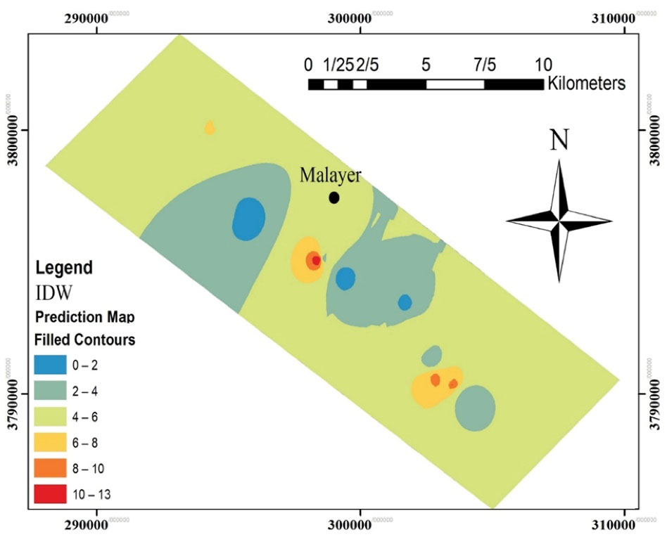
Figure 2.
Interpolated Map for Contamination with Copper.
.
Interpolated Map for Contamination with Copper.
Generally, 2-4 concentration class accounted for the majority of the area in the study area. There are centers with a high concentration of contamination in the northwest, center, and southeast of the study area as well as in the intervals between the pollution centers of the regions with low contamination. The determination of the spatial distribution of contamination enabled the investigation of the effects of various spatial factors.
3.5. Land Use
Fig. 3 demonstrates the LUM. According to the field studies, the investigation of the high-quality images available in Google Earth and validation works, the generated LUM was found to match the ground truths in the study area. Based on the obtained results, the most frequent land-use types in the vicinity of the vineyards in the northwestern and central sections of the study area were adobe furnace, residential and agricultural. Additionally, the agricultural and residential activities account for the majority of the land uses in the southeastern side of the study area.
It is evident from the comparison of the spatial distribution map of copper contamination with the LUM that the contamination centers matched some land uses. The pollution center in the northwest of the study area matched the residential and adobe furnace land-use types. Moreover, the pollution center in the center of the study area matched the residential and adobe furnace land-use types and the pollution center in the southeast of the study area matched the residential land use. In general, the contamination rate decreased with an increase in the distance from the residential sites and adobe furnaces.
4. Conclusion
The soil of vineyards in Malayer was contamination with copper. The results obtained for Cf and Igeo indices were indicative of the idea that the soils were moderately contaminated with metals. It can be found out in a comparison of the interpolation map of copper contamination and the LUM that the contamination was higher in the places with residential sites and adobe furnaces. As can be observed in the maps, the contamination was higher in the vineyards on the periphery of Malayer and Gurab; this could be because of air pollution originating from activities in the residential regions and adobe furnaces. It was made clear in the field investigations and inquiring the farmers and sellers of the chemicals and fertilizers that the farmers were using copper-containing pesticides, which can also be another source of the contamination of the vineyard soil with copper.
Generally, the potential ecological risk index for the studied metals in the region and the total ecological risk were at a low level. Moreover, the copper accumulation in grapevine species was found to be lower in comparison with the other studied elements in the present study. This originated from the positive correlation of the physiological properties of the grapevine species with the environmental conditions, including the low concentration of the metals in the study area. Considering copper contamination, the low accumulation of the grapevine species did not cause a reduction in the product quality in these vineyards. However, the situation can be dangerous considering the fact that this amount of copper contamination has come about within a short period of time and further studies are required for managing and controlling the pollution. In these studies, the source and control method of copper contamination and product quality with respect to copper contamination as well as the grapevine properties should be investigated under various contingent conditions.
Conflict of Interests
The authors declare that they have no conflict of interests.
Acknowledgements
We highly appreciate the efforts and cooperation of Mustafa Mirshahvald, the head of the Central Laboratory, Bahar Roozbahani and Farnaz Mahmoodi lab manager of the University of Malayer.
Author’s Contribution
MP:Sampling, Sample perpetration, Investigation, Software & Writing
SM:Methodology, Sample Analysis, Supervision, Writing - review & editing.
References
- Wei B, Yang L. A review of heavy metal contaminations in urban soils, urban road dusts and agricultural soils from China. Microchem J 2010; 94(2):99-107. doi: 10.1016/j.microc.2009.09.014 [Crossref] [ Google Scholar]
- Altaş L. Inhibitory effect of heavy metals on methane-producing anaerobic granular sludge. J Hazard Mater 2009; 162(2-3):1551-6. doi: 10.1016/j.jhazmat.2008.06.048 [Crossref] [ Google Scholar]
- Keller A, von Steiger B, van der Zee SE, Schulin R. A stochastic empirical model for regional heavy-metal balances in agroecosystems. J Environ Qual 2001; 30(6):1976-89. doi: 10.2134/jeq2001.1976 [Crossref] [ Google Scholar]
- Huang SW, Jin JY. Status of heavy metals in agricultural soils as affected by different patterns of land use. Environ Monit Assess 2008; 139(1-3):317-27. doi: 10.1007/s10661-007-9838-4 [Crossref] [ Google Scholar]
- Orescanin V, Katunar A, Kutle A, Valkovic V. Heavy metals in soil, grape, and wine. Journal of Trace and Microprobe Techniques 2003; 21(1):171-80. doi: 10.1081/TMA-120017912 [Crossref] [ Google Scholar]
- Bălc R, Tămaş T, Popita GE, Vasile GG, Bratu MC, Gligor DM. Assessment of chemical elements in soil, grapes and wine from two representative vineyards in Romania. Carpath J Earth Environ Sci 2018; 13(2):435-46. doi: 10.26471/cjees/2018/013/037 [Crossref] [ Google Scholar]
- Beygi M, Jalali M. Assessment of trace elements (Cd, Cu, Ni, Zn) fractionation and bioavailability in vineyard soils from the Hamedan, Iran. Geoderma 2019; 337:1009-20. doi: 10.1016/j.geoderma.2018.11.009 [Crossref] [ Google Scholar]
- Bravo S, Amorós JA, Pérez-de-los-Reyes C, García FJ, Moreno MM, Sánchez-Ormeño M. Influence of the soil pH in the uptake and bioaccumulation of heavy metals (Fe, Zn, Cu, Pb and Mn) and other elements (Ca, K, Al, Sr and Ba) in vine leaves, Castilla-La Mancha (Spain). J Geochem Explor 2017; 174:79-83. doi: 10.1016/j.gexplo.2015.12.012 [Crossref] [ Google Scholar]
- Gallo A, Zannoni D, Valotto G, Nadimi-Goki M, Bini C. Concentrations of potentially toxic elements and soil environmental quality evaluation of a typical Prosecco vineyard of the Veneto region (NE Italy). J Soils Sediments 2018; 18(11):3280-9. doi: 10.1007/s11368-018-1999-y [Crossref] [ Google Scholar]
- Li X, Dong S, Su X. Copper and other heavy metals in grapes: a pilot study tracing influential factors and evaluating potential risks in China. Sci Rep 2018; 8(1):17407. doi: 10.1038/s41598-018-34767-z [Crossref] [ Google Scholar]
- Milićević T, Relić D, Urošević MA, Vuković G, Škrivanj S, Samson R. Integrated approach to environmental pollution investigation - spatial and temporal patterns of potentially toxic elements and magnetic particles in vineyard through the entire grapevine season. Ecotoxicol Environ Saf 2018; 163:245-54. doi: 10.1016/j.ecoenv.2018.07.078 [Crossref] [ Google Scholar]
- Solgi I, Solgi M. Investigating of heavy metals concentration Vineyard soils in the agricultural ecosystems of Malayer. Journal of Plant Ecosystem Conservation 2016; 3(7):99-112. [ Google Scholar]
- FAO. Grape production system in Jowzan.Food and Agriculture Organization of the United Nations: GIAHS; 2018. Available from: http://www.fao.org/giahs/giahsaroundtheworld/designated-sites/near-east-and-north-africa/grape-production-system-in-jowzan-valley/en/.
- Jalali M, Kolahchi Z. Groundwater quality in an irrigated, agricultural area of northern Malayer, western Iran. Nutr Cycl Agroecosys 2008; 80(1):95-105. doi: 10.1007/s10705-007-9123-5 [Crossref] [ Google Scholar]
- Bowen HJM. Environmental Chemistry of the Elements. London: Academic Press; 1979.
- Mason B, Moore CB. Principles of Geochemistry. New York: John Wiley & Sons;1966. p. 471–57521.
- Turekian KK, Wedepohl KH. Distribution of the elements in some major units of the earth’s crust. Geol Soc Am Bull 1961; 72(2):175-92. doi: 10.1130/0016-7606(1961)72[175:DOTEIS]2.0.CO;2 [Crossref] [ Google Scholar]
- Hakanson L. An ecological risk index for aquatic pollution control A sedimentological approach. Water Res 1980; 14(8):975-1001. doi: 10.1016/0043-1354(80)90143-8 [Crossref] [ Google Scholar]
- Muller G. Index of geoaccumulation in sediments of the Rhine River. GeoJournal 1969; 2(3):108-18. [ Google Scholar]
- Lu A, Wang J, Qin X, Wang K, Han P, Zhang S. Multivariate and geostatistical analyses of the spatial distribution and origin of heavy metals in the agricultural soils in Shunyi, Beijing, China. Sci Total Environ 2012; 425:66-74. doi: 10.1016/j.scitotenv.2012.03.003 [Crossref] [ Google Scholar]
- Kabata-Pendias A. Trace Elements in Soils and Plants. Boca Raton, Florida: CRC Press; 2010.
- Chen Y, Jiang X, Wang Y, Zhuang D. Spatial characteristics of heavy metal pollution and the potential ecological risk of a typical mining area: A case study in China. Process Saf Environ Prot 2018; 113:204-19. doi: 10.1016/j.psep.2017.10.008 [Crossref] [ Google Scholar]
- Gong G, Mattevada S, O’Bryant SE. Comparison of the accuracy of kriging and IDW interpolations in estimating groundwater arsenic concentrations in Texas. Environ Res 2014; 130:59-69. doi: 10.1016/j.envres.2013.12.005 [Crossref] [ Google Scholar]
- Gotway CA, Ferguson RB, Hergert GW, Peterson TA. Comparison of kriging and inverse-distance methods for mapping soil parameters. Soil Sci Soc Am J 1996; 60(4):1237-47. doi: 10.2136/sssaj1996.03615995006000040040x [Crossref] [ Google Scholar]
- Spokas K, Graff C, Morcet M, Aran C. Implications of the spatial variability of landfill emission rates on geospatial analyses. Waste Manag 2003; 23(7):599-607. doi: 10.1016/s0956-053x(03)00102-8 [Crossref] [ Google Scholar]
- Wartenberg D, Uchrin C, Coogan P. Estimating exposure using kriging: a simulation study. Environ Health Perspect 1991; 94:75-82. doi: 10.1289/ehp.94-1567973 [Crossref] [ Google Scholar]
- Zhou Y, Michalak AM. Characterizing attribute distributions in water sediments by geostatistical downscaling. Environ Sci Technol 2009; 43(24):9267-73. doi: 10.1021/es901431y [Crossref] [ Google Scholar]
- Webster R, Oliver MA. Geostatistics for Environmental Scientists. John Wiley & Sons; 2007.
- Schulz JJ, Cayuela L, Echeverria C, Salas J, Rey Benayas JM. Monitoring land cover change of the dryland forest landscape of Central Chile (1975–2008). Appl Geogr 2010; 30(3):436-47. doi: 10.1016/j.apgeog.2009.12.003 [Crossref] [ Google Scholar]
- Song C, Woodcock CE, Seto KC, Lenney MP, Macomber SA. Classification and change detection using Landsat TM data: when and how to correct atmospheric effects?. Remote Sens Environ 2001; 75(2):230-44. doi: 10.1016/S0034-4257(00)00169-3 [Crossref] [ Google Scholar]
- McIver DK, Friedl MA. Using prior probabilities in decision-tree classification of remotely sensed data. Remote Sens Environ 2002; 81(2-3):253-61. doi: 10.1016/S0034-4257(02)00003-2 [Crossref] [ Google Scholar]
- Rosenfield GH, Fitzpatrick-Lins K. A coefficient of agreement as a measure of thematic classification accuracy. Photogramm Eng Remote Sensing 1986; 52(2):223-7. [ Google Scholar]
- Mohammadian Mosammam H, Tavakoli Nia J, Khani H, Teymouri A, Kazemi M. Monitoring land use change and measuring urban sprawl based on its spatial forms: the case of Qom city. Egypt J Remote Sens Space Sci 2017; 20(1):103-16. doi: 10.1016/j.ejrs.2016.08.002 [Crossref] [ Google Scholar]
- Chaignon V, Sanchez-Neira I, Herrmann P, Jaillard B, Hinsinger P. Copper bioavailability and extractability as related to chemical properties of contaminated soils from a vine-growing area. Environ Pollut 2003; 123(2):229-38. doi: 10.1016/s0269-7491(02)00374-3 [Crossref] [ Google Scholar]
- Bhuiyan MAH, Parvez L, Islam MA, Dampare SB, Suzuki S. Heavy metal pollution of coal mine-affected agricultural soils in the northern part of Bangladesh. J Hazard Mater 2010; 173(1-3):384-92. doi: 10.1016/j.jhazmat.2009.08.085 [Crossref] [ Google Scholar]
- Li X, Feng L. Multivariate and geostatistical analyzes of metals in urban soil of Weinan industrial areas, Northwest of China. Atmospheric Environment 2012; 47:58-65. doi: 10.1016/j.atmosenv.2011.11.041 [Crossref] [ Google Scholar]