Avicenna J Environ Health Eng. 10(1):38-43.
doi: 10.34172/ajehe.2023.5376
Original Article
Predictive Modeling for Forecasting Air Quality Index (AQI) Using Time Series Analysis
Alka Pant 1, *  , Ramesh Chandra Joshi 2 , Sanjay Sharma 3 , Kamal Pant 4
Author information:
1School of Computing, Graphic Era Hill University, Dehradun, Uttarakhand, India
2Department of Computer Science and Engineering, School of Engineering, Graphic Era (Deemed to be University), Dehradun, Uttarakhand, India
3Department of Computer Applications, School of Computer Applications and Information Technology, Shri Guru Ram Rai University, Dehradun, Uttarakhand, India
4School of Vocational Studies, Graphic Era Hill University, Dehradun, Uttarakhand, India
Abstract
Air pollution is a widespread problem in India. The study focuses on forecasting the air quality index (AQI) using time series modeling techniques for the most polluted area of Dehradun City in Uttarakhand state, India. The train test approach of machine learning and Akaike information criterion (AIC) have been used on the monthly data of five years to select the best auto-regressive model. Using the auto-correlation functions (ACF and PACF) and the seasonality component in the time-series dataset, a seasonal auto-regressive moving average (ARMA) model with its minimum AIC has been chosen to forecast the AQI. This model is also validated by comparing its predicted values with the actual values of AQI. The results showed that the seasonal ARMA model of (1,0,0)(1,0,0)12 could forecast AQI based on a stationary dataset. The research also indicates that the asthma patients of the Himalayan Drugs-ISBT region may experience more health effects, especially in winter, due to poor air quality. The model can be helpful for a scientist and the government to take precautionary measures in advance.
Keywords: Air quality index, Time series analysis, Auto-correlation, Seasonal ARMA, Forecasting,
Copyright and License Information
© 2023 The Author(s); Published by Hamadan University of Medical Sciences.
This is an open-access article distributed under the terms of the Creative Commons Attribution License (
https://creativecommons.org/licenses/by/4.0), which permits unrestricted use, distribution, and reproduction in any medium, provided the original work is properly cited.
Please cite this article as follows: Pant A, Joshi RC, Sharma S, Pant K. Predictive modeling for forecasting air quality index (AQI) using time series analysis. Avicenna J Environ Health Eng. 2023; 10(1):38-43. doi:10.34172/ajehe.2023.5376
1. Introduction
Any activity leading to degradation by violating the original nature of the environment is called pollution (1). After the industrial revolution, things deteriorated considerably, marking the rapid growth in the number of industries and automobiles that contributed significantly to air pollution. The air quality index (AQI) is a quantitative indicator of air quality in a region. There are six AQI categories, namely good, satisfactory, moderately polluted, poor, very poor, and severe. There was an improvement in air pollution during the lockdown period of the pandemic (COVID-19) across the globe because of the restricted emissions from different sources (2). Air pollution is a widespread problem in developing countries such as India, and machine learning algorithms are essential tools for predicting the AQI value (3). Based on past values, knowing future AQI values in different regions is necessary. Time series analysis makes it easier as it is an application of data science using the time parameter (4). In past studies, researchers employed various strategies to predict the value of AQI using machine learning algorithms such as logistic regression, random forest, and decision trees (5-7). Some researchers also developed their models through the artificial neural network and regression techniques for forecasting and prediction of AQI (8,9). To forecast the AQI, an autoregressive model (i.e., ARIMA) can also be used (10). Therefore, this study aimed to predict an effective model to forecast the values of the AQI using time series analysis for the most polluted region.
2. Materials and Methods
The autoregressive models used in time-series forecasting is essential in monitoring and controlling air quality condition. These models are based on the assumption that the future values of the AQI will resemble its past dataset. The appropriate visualization of data is also required to set a prediction model for the AQI. Python language with Matplot and Pmdarima libraries is used for data visualization. To forecast the AQI for twelve months, we have tried to find the appropriate model to predict the AQI using the time series technique in the Jupyter notebook. We have chosen the region of Himalayan Drugs Company considering that it is the most polluted area of Dehradun city, the capital of Uttarakhand state. This region is located near the Inter-State Bus Terminus (ISBT) of this city. AQI values of 5 years were obtained from the Uttarakhand Government (CPCB) for predictive modelling purposes and were used to forecast the AQI values. We have used the decomposition process to see the trend and seasonality components of our dataset. The Dickey-Fuller test has also been used to know the status (stationary or non-stationary) in our time series dataset.
2.1. Decomposition of a Time Series
A time series is an ordered list of observations made at predefined time intervals. The observation of the time series cannot be independent of each other. Adjusting trend and seasonality components in the data set decomposition and differencing is applied. The decomposition process breaks down the original time series into its components, including a trend (T), seasonality (S), cyclic (C), and residual (R), and studies each component separately.
2.2. Stationarity of the Time Series
The time series forecasting methods are best fitted to a stationary time series. Therefore, the first step in applying the time series forecasting models is to check whether the series is stationary. The Dickey-Fuller test is the most commonly and frequently used statistical method to test stationarity (11). An auto-correlation function (ACF) plot can also be used to identify the status of a time series. If a series is not stationary, then it will be made as a stationary series to stabilize the mean values through the differencing process.
2.3. Time Series Modeling Techniques
2.3.1. Auto-Regressive Model
Auto-regressive (AR) model refers to a model where the dependent variable is the current value and the independent variables are N previous values of the time series. AR model considers past values and error terms for predicting future value. AR models are called the long memory model as the first observation of the series always somehow affects the current value of the variable irrespective of the time. The primary assumption for estimating the time series is that the correlation with the increase in lags should decrease, so the impact should be highest for the first lag and slowly diminish to zero. A time series of ‘p’ past values with error is called AR (p). The model that only depends on the previous value of the previous lag or one lag in the past is called AR(1).
2.3.2. Moving Average Model
Moving average (MA) model refers to a model in which the variable does not depend on any other variable. Instead, it depends on the lag of error. In this model, we estimate the future value based solely on past errors in the series. The value of error is the difference between the expected value and the actual value in the past. It is based on the assumption that the literal error from the past time affects the current value. MA model is also called the short memory model because these errors do not last long into the future. A time series of q past errors is called MA (q).
2.3.3. ARMA or ARIMA
Auto-regressive integrated moving average (ARIMA) model is used when a time series is non-stationary, whereas the auto-regressive moving average (ARMA) is used when the variable in a series is stationary. In ARMA or ARIMA modeling, we can find out how many orders the AR and MA go up through the ACF (q) and partial ACF (p). In ARIMA, ‘I’ means integrated, which indicates that the original series has already been transformed into a stationary one through the differencing process. If a time series has a seasonality component, seasonal ARMA or seasonal ARIMA (SARIMA) will be used (12). Similar to ARIMA, the SARIMA model also considers the p, d, and q parameters. SARIMA also includes seasonal components: P, D, Q, and m parameters. Here, P means seasonal auto-regressive, D means the order of seasonal differencing, Q means the seasonal moving average, and m is the number of seasonal periods (13,14).
2.4. ACF and PACF
The ACF allows the experts to compare the current value of the dataset to its historical value. Therefore, auto-correlation means the correlation between two variables at a specified point in the time series, and its function can be more understandable with the help of a graph. The ACF plot can quickly determine the pattern of trend and seasonality. The partial auto-correlation function (PACF) only considers the direct effect between two dataset observations. The PACF plot is used to specify regression models with time series data and the ARIMA model. The ACF and PACF determine the order of p and q, whose values are utilized in the auto-regressive model (15).
2.5. Akaike Information Criterion
To validate an auto-regressive model, the Akaike information criterion(AIC) has been used (16). The favored model is the one with the minimum AIC value. With the help of AIC, a data scientist can select the model that minimizes the estimated information loss.
3. Results and Discussion
The time series techniques were used to predict a model for forecasting the AQI values for the region of Himalayan Drugs-ISBT in Dehradun city. For this purpose, 60 valid data points (2017-2021) have been collected from the State Government’s Central Pollution Control Board (CPCB). Auto-regressive models implicitly assume that the future will resemble the past, which means predicted future values are based on past values. Therefore, an auto-regressive model was developed and the fitting effect of this model was verified (17). Using the train test approach of machine learning, we split our data points into a training dataset and a test dataset (18). In this study, AQI values of four years (2017, 2018, 2019 & 2020) were taken as the training dataset and the rest (2021) as the test dataset. The auto-regressive model is best fitted on a stationary time series dataset. As a preliminary step of our work, we checked out the stationarity of our dataset to find out whether our AQI dataset was stationary or not. We investigated this with the help of the augmented Dickey-Fuller test (19). Here, the P value (0.003) was less than the significance level (0.05), indicating that our AQI dataset was a stationary dataset, so there was no need for differencing. Fig. 1 also shows a stationary time series of our dataset due to the missing trend. It is also clear from our ACF plot (Fig. 2) because we know that in the case of a non-stationary dataset, there is a significant spike at lag 1, which slowly decreases over several lags (20).
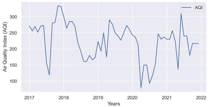
Fig. 1.
Time Series of AQI Dataset for Himalayan Drugs-ISBT Region
.
Time Series of AQI Dataset for Himalayan Drugs-ISBT Region
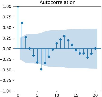
Fig. 2.
Auto-correlation (ACF) Plot
.
Auto-correlation (ACF) Plot
The next step was to select the auto-regressive model to forecast the AQI for the most polluted area of Dehradun city located in the region of Himalayan Drugs-ISBT. Based on the stationarity of the dataset, many researchers have used the ARMA or ARIMA model to forecast the AQI (21-23). The seasonal component is an essential factor in choosing the best auto-regressive model. Therefore, we first had to check the seasonality component in our AQI dataset. For this purpose, we decomposed our time series dataset into trend, seasonal, and residual components (Fig. 3). Here, we identified the seasonal component in our AQI dataset, which validated that the seasonal ARMA model could best forecast the AQI.
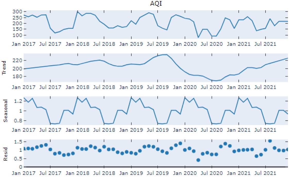
Fig. 3.
Time Series Decomposition of AQI Dataset
.
Time Series Decomposition of AQI Dataset
Based on the seasonality component of the stationary time series AQI dataset, the next step was to finalize the order [(p, q) and (P, Q)] of our seasonal ARMA model. We have already plotted the ACF and PACF plots to figure out the seasonal order of P(AR) and Q(MA) parameters. Figs. 2 and 4 indicate that P(AR) and Q(MA) can be 1.
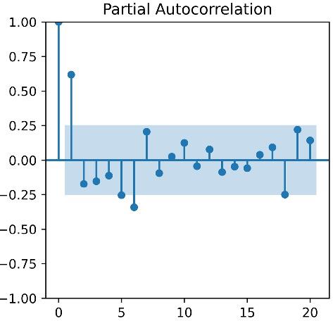
Fig. 4.
Partial Auto-correlation (PACF) Plot
.
Partial Auto-correlation (PACF) Plot
At last, we used the Pmdarima library in the same language (Python language), which could provide the best order based on their minimum AIC. According to the AIC criterion, the smaller the AIC value, the better the fitting effect of the model. Table 1 shows different parameters {(p, d, q) (P, D, Q), [m]} of the seasonal ARMA model with their AIC values provided by the Pmdarima library (24). Here, many experiments have been performed several times. It was concluded that the seasonal ARMA (1,0,0) (1,0,0), [12] model with a minimum AIC value of 630.19 comprised the best parameters (p, q and P, Q) to forecast the AQI.
Table 1.
SARIMA Model Fitting Results
Seasonal ARMA Model
(p, d, q) (P, D, Q) [m]
|
Evaluation Parameter
(AIC Values)
|
| ARMA(1,0,1)(0,0,0) [12] |
632.95 |
| ARMA(1,0,0)(1,0,0) [12] |
630.19 |
| ARMA(0,0,1)(0,0,1) [12] |
634.90 |
| ARMA(1,0,0)(2,0,0) [12] |
631.51 |
| ARMA(0,0,0)(1,0,0) [12] |
653.70 |
| ARMA(2,0,0)(1,0,0) [12] |
630.62 |
To forecast the AQI for the next 12 months, we have taken the values up to December 2020 as a training dataset and January 2021 as a test dataset for validation purposes. Using the seasonal ARMA {(1,0,0) (1,0,0), [12]} model, predicted values have been calculated for the test dataset. We have plotted these predicted values with our actual (test) dataset for the model validation purpose, and it seemed quite acceptable to refit the entire dataset (Fig. 5).
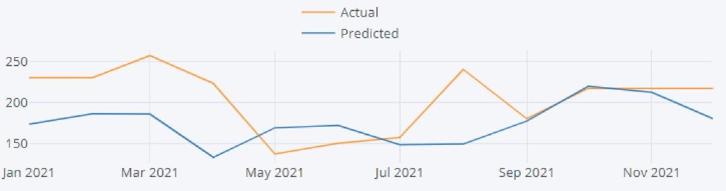
Fig. 5.
Test Versus Predicted AQI Values Using Seasonal ARMA Model
.
Test Versus Predicted AQI Values Using Seasonal ARMA Model
After this validation process of the model, the last step was to forecast the AQI values for 12 months. Table 2 and Fig. 6 show the forecasted AQI values for the following year.
Table 2.
Forecast Values of AQI
|
Date
|
Forecast Values
|
| 2022-01-01 |
227.77 |
| 2022-02-01 |
222.15 |
| 2022-03-01 |
226.36 |
| 2022-04-01 |
214.94 |
| 2022-05-01 |
189.83 |
| 2022-06-01 |
192.78 |
| 2022-07-01 |
194.33 |
| 2022-08-01 |
217.22 |
| 2022-09-01 |
200.36 |
| 2022-10-01 |
210.59 |
| 2022-11-01 |
210.54 |
| 2022-12-01 |
210.51 |
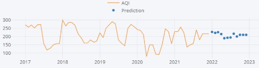
Fig. 6.
Forecast of AQI Values Using Seasonal ARMA Model
.
Forecast of AQI Values Using Seasonal ARMA Model
Fig. 7 shows a predictive model based on the seasonal ARMA model for forecasting the AQI for a stationary time series dataset.
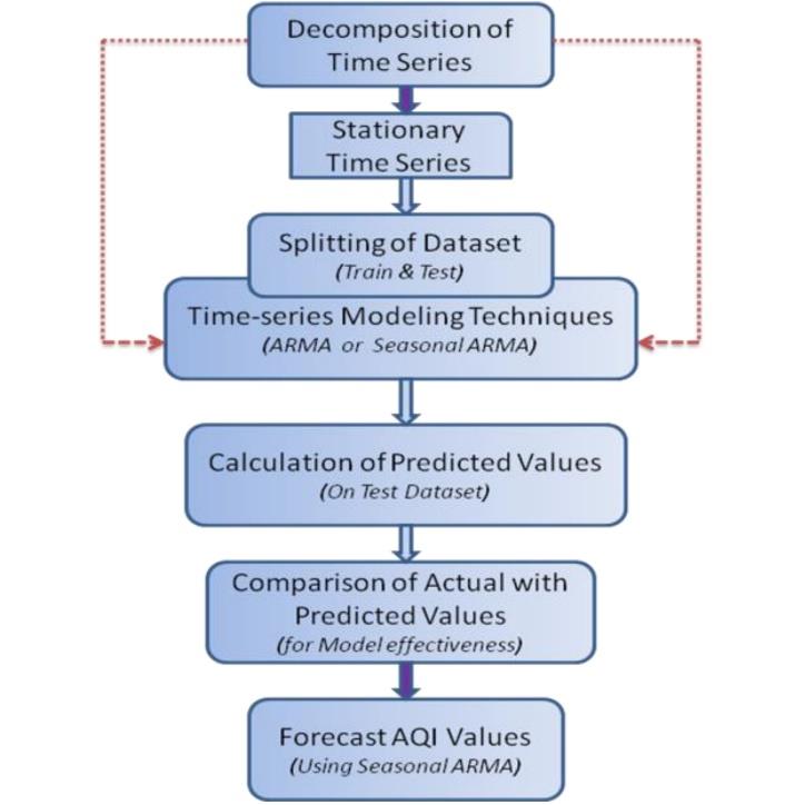
Fig. 7.
Predictive Model for AQI Forecasting
.
Predictive Model for AQI Forecasting
4. Conclusion
Polluted air can be seen in every state of India, but we can forecast the upcoming air pollution trends using historical information and experiences. For predicting air quality, machine learning has made incredible technological breakthroughs. This paper presented a predictive model to forecast the AQI level for the most polluted region of Dehradun City using the time series auto-regression technique. Due to the seasonal component in the stationary time series dataset and with the help of the auto ARIMA function in Python language, a seasonal ARMA model of {(1,0,0) (1,0,0), [12]} has been selected based on its minimum AIC. However, the mean absolute error and root mean square error can also be used in the near future. This model of seasonal ARMA can also be validated in this study, as the predicted values of AQI are based on the actual values of the test dataset. After the validation process, the values of AQI were forecasted for the next 12 months. The research also indicates that the sensitive persons (asthma patients) of the Himalayan Drugs-ISBT region may experience health issues, especially in winter, due to poor air quality. The model can be helpful for a scientist, and the forecasted values of AQI for this region can help the government to develop effective policies.
Author’s Contribution
Conceptualization: Alka Pant, Ramesh Chandra Joshi.
Data curation: Alka Pant.
Formal analysis: Alka Pant.
Methodology: Alka Pant, Ramesh Chandra Joshi.
Supervision: Ramesh Chandra Joshi, Sanjay Sharma.
Validation: Sanjay Sharma; Alka Pant, Kamal Pant.
Visualization: Alka Pant; Kamal Pant.
Writing–original draft: Alka Pant, Sanjay Sharma.
Writing–review & editing: Alka Pant, Ramesh Chandra Joshi, Kamal Pant.
Competing Interests
The authors have declared that no competing interests exist.
Funding
In this research, no grants were received by the authors.
References
- Torkashvand J, Azarian G, Leili M, Godini K, Younesi S, Godini H. Projection of environmental pollutant emissions from different final waste disposal methods based on life cycle assessment studies in Qazvin city. Avicenna J Environ Health Eng 2015; 2(2):4653. doi: 10.17795/ajehe-4653 [Crossref] [ Google Scholar]
- Manisalidis I, Stavropoulou E, Stavropoulos A, Bezirtzoglou E. Environmental and health impacts of air pollution: a review. Front Public Health 2020; 8:14. doi: 10.3389/fpubh.2020.00014 [Crossref] [ Google Scholar]
- Pant A, Sharma S, Joshi R. Air quality modeling for effective environmental management in Uttarakhand, India: a comparison of logistic regression and naive bayes. J Air Pollut Health 2022; 7(3):287-98. doi: 10.18502/japh.v7i3.10542 [Crossref] [ Google Scholar]
- Sethi JK, Mittal M. Analysis of air quality using univariate and multivariate time series models. In: 2020 10th International Conference on Cloud Computing, Data Science & Engineering (Confluence). Noida, India: IEEE; 2020. p. 823-7. 10.1109/Confluence47617.2020.9058303.
- Pant A, Sharma S, Bansal M, Narang M. Comparative analysis of supervised machine learning techniques for AQI prediction. In: 2022 International Conference on Advanced Computing Technologies and Applications (ICACTA). Coimbatore, India: IEEE; 2022. p. 1-4. 10.1109/icacta54488.2022.9753636.
- Pal S, Pramanik D, Jain E. Effectiveness of machine learning algorithms in forecasting AQI. In: 2021 International Conference on Technological Advancements and Innovations (ICTAI). Tashkent, Uzbekistan: IEEE; 2021. p. 492-5. 10.1109/ictai53825.2021.9673385.
- Bhalgat P, Pitale S, Bhoite S. Air quality prediction using machine learning algorithms. Int J Comput Appl Technol Res 2019; 8(9):367-70. doi: 10.7753/ijcatr0809.1006 [Crossref] [ Google Scholar]
- Jiang D, Zhang Y, Hu X, Zeng Y, Tan J, Shao D. Progress in developing an ANN model for air pollution index forecast. Atmos Environ 2004; 38(40):7055-64. doi: 10.1016/j.atmosenv.2003.10.066 [Crossref] [ Google Scholar]
- Ganesh SS, Modali SH, Palreddy SR, Arulmozhivarman P. Forecasting air quality index using regression models: a case study on Delhi and Houston. In: 2017 International Conference on Trends in Electronics and Informatics (ICEI). Tirunelveli, India: IEEE; 2017. p. 248-54. 10.1109/icoei.2017.8300926.
- Liu T, You S. Analysis and forecast of Beijing’s air quality index based on ARIMA model and neural network model. Atmosphere 2022; 13(4):512. doi: 10.3390/atmos13040512 [Crossref] [ Google Scholar]
- Dickey DA, Fuller WA. Distribution of the estimators for autoregressive time series with a unit root. J Am Stat Assoc 1979; 74(366a):427-31. doi: 10.1080/01621459.1979.10482531 [Crossref] [ Google Scholar]
- Bhagat J, Saha G. Pollutant PM2.5 multi step prediction under seasonal influences across 13 Indian cities. In: 2021 Innovations in Power and Advanced Computing Technologies (i-PACT). Kuala Lumpur, Malaysia: IEEE; 2021. p. 1-8. 10.1109/i-PACT52855.2021.9696866.
- Maltare NN, Vahora S. Air quality index prediction using machine learning for Ahmedabad city. Digital Chemical Engineering 2023; 7:100093. doi: 10.1016/j.dche.2023.100093 [Crossref] [ Google Scholar]
- Hyndman RJ, Athanasopoulos G. Forecasting: Principles and Practice. 3rd ed. Melbourne, Australia: OTexts; 2021.
- Saleh I, Abedi S, Abedi S, Bastani M, Beman E. Developing a model to predict air pollution (case study: Tehran city). J Environ Health Sci Eng 2021; 19(1):71-80. doi: 10.1007/s40201-020-00582-w [Crossref] [ Google Scholar]
- Akaike H. Information theory and an extension of the maximum likelihood principle. In: Parzen E, Tanabe K, Kitagawa G, eds. Selected Papers of Hirotugu Akaike. New York, NY: Springer; 1998. p. 199-213. 10.1007/978-1-4612-1694-0_15.
- Singh R, Singh V, Sharma N. US air quality index forecasting: a comparative study. In: Batra U, Roy N, Panda B, eds. Data Science and Analytics: 5th International Conference on Recent Developments in Science, Engineering and Technology, Gurugram, India. Singapore: Springer; 2020. p. 91-102. 10.1007/978-981-15-5827-6_8.
- Senthivel S, Chidambaranathan M. Machine learning approaches used for air quality forecast: a review. Rev Intell Artif 2022; 36(1):73-8. doi: 10.18280/ria.360108 [Crossref] [ Google Scholar]
- Barthwal A, Acharya D. An IoT based sensing system for modeling and forecasting urban air quality. Wirel Pers Commun 2021; 116(4):3503-26. doi: 10.1007/s11277-020-07862-6 [Crossref] [ Google Scholar]
- Nimesh R, Arora S, Mahajan KK, Gill AN. Predicting air quality using ARIMA, ARFIMA and HW smoothing. Model Assist Stat Appl 2014; 9(2):137-49. doi: 10.3233/mas-130285 [Crossref] [ Google Scholar]
- Taneja K, Ahmad S, Ahmad K, Attri SD. Time series analysis of aerosol optical depth over New Delhi using Box–Jenkins ARIMA modeling approach. Atmos Pollut Res 2016; 7(4):585-96. doi: 10.1016/j.apr.2016.02.004 [Crossref] [ Google Scholar]
- Tomar N, Patel D, Jain A. Air quality index forecasting using auto-regression models. In: 2020 IEEE International Students’ Conference on Electrical, Electronics and Computer Science (SCEECS). Bhopal, India: IEEE; 2020. p. 1-5. 10.1109/sceecs48394.2020.216.
- Mani G, Viswanadhapalli JK, Stonier AA. Prediction and forecasting of air quality index in Chennai using regression and ARIMA time series models. J Eng Res 2022; 10(2A):179-94. doi: 10.36909/jer.10253 [Crossref] [ Google Scholar]
- Lee MH, Abd Rahman NH, Suhartono Suhartono, Latif MT, Nor ME, Kamisan NA. Seasonal ARIMA for forecasting air pollution index: a case study. Am J Appl Sci 2012; 9(4):570-8. doi: 10.3844/ajassp.2012.570.578 [Crossref] [ Google Scholar]